【python数据挖掘课程】十.Pandas、Matplotlib、PCA绘图实用代码补充
2017-03-07 15:24
981 查看
这篇文章主要是最近整理《数据挖掘与分析》课程中的作品及课件过程中,收集了几段比较好的代码供大家学习。同时,做数据分析到后面,除非是研究算法创新的,否则越来越觉得数据非常重要,才是有价值的东西。后面的课程会慢慢讲解Python应用在Hadoop和Spark中,以及networkx数据科学等知识。
如果文章中存在错误或不足之处,还请海涵~希望文章对你有所帮助。
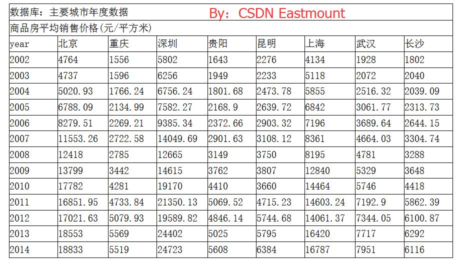
数据集位32.csv,具体值如下:(读者可直接复制)
year Beijing Chongqing Shenzhen Guiyang Kunming Shanghai Wuhai Changsha
2002 4764.00 1556.00 5802.00 1643.00 2276.00 4134.00 1928.00 1802.00
2003 4737.00 1596.00 6256.00 1949.00 2233.00 5118.00 2072.00 2040.00
2004 5020.93 1766.24 6756.24 1801.68 2473.78 5855.00 2516.32 2039.09
2005 6788.09 2134.99 7582.27 2168.90 2639.72 6842.00 3061.77 2313.73
2006 8279.51 2269.21 9385.34 2372.66 2903.32 7196.00 3689.64 2644.15
2007 11553.26 2722.58 14049.69 2901.63 3108.12 8361.00 4664.03 3304.74
2008 12418.00 2785.00 12665.00 3149.00 3750.00 8195.00 4781.00 3288.00
2009 13799.00 3442.00 14615.00 3762.00 3807.00 12840.00 5329.00 3648.00
2010 17782.00 4281.00 19170.00 4410.00 3660.00 14464.00 5746.00 4418.00
2011 16851.95 4733.84 21350.13 5069.52 4715.23 14603.24 7192.90 5862.39
2012 17021.63 5079.93 19589.82 4846.14 5744.68 14061.37 7344.05 6100.87
2013 18553.00 5569.00 24402.00 5025.00 5795.00 16420.00 7717.00 6292.00
2014 18833.00 5519.00 24723.00 5608.00 6384.00 16787.00 7951.00 6116.00
绘制对比各个城市的商品房价数据代码如下所示:
# -*- coding: utf-8 -*-
"""
Created on Mon Mar 06 10:55:17 2017
@author: eastmount
"""
import pandas as pd
data = pd.read_csv("32.csv",index_col='year') #index_col用作行索引的列名
#显示前6行数据
print(data.shape)
print(data.head(6))
import matplotlib.pyplot as plt
plt.rcParams['font.sans-serif'] = ['simHei'] #用来正常显示中文标签
plt.rcParams['axes.unicode_minus'] = False #用来正常显示负号
data.plot()
plt.savefig(u'时序图.png', dpi=500)
plt.show()
输出如下所示:
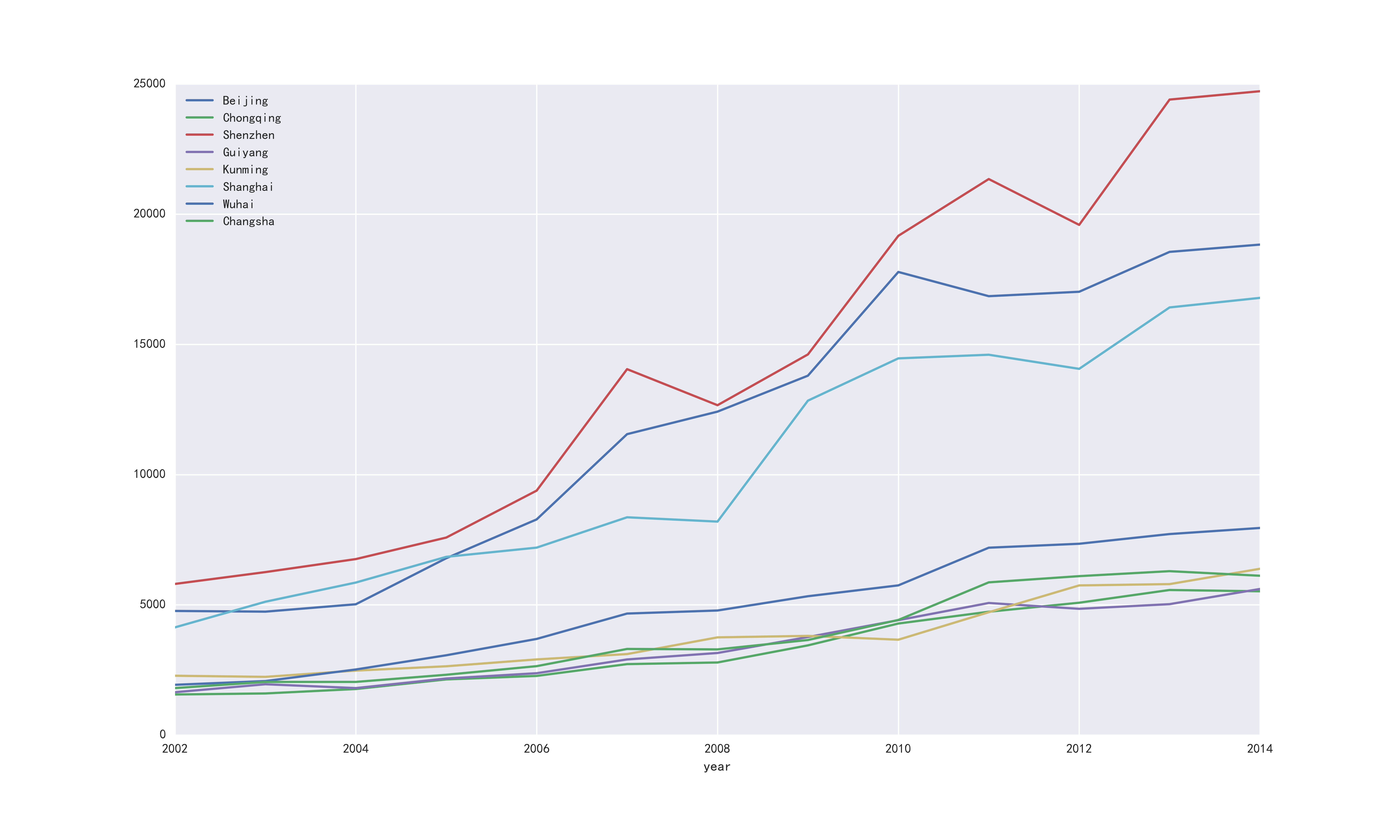
重点知识:
1、plt.rcParams显示中文及负号;
2、plt.savefig保存图片至本地;
3、pandas直接读取数据显示绘制图形,index_col获取索引。
# -*- coding: utf-8 -*-
"""
Created on Mon Mar 06 10:55:17 2017
@author: eastmount
"""
import pandas as pd
data = pd.read_csv("32.csv",index_col='year') #index_col用作行索引的列名
#显示前6行数据
print(data.shape)
print(data.head(6))
import matplotlib.pyplot as plt
plt.rcParams['font.sans-serif'] = ['simHei'] #用来正常显示中文标签
plt.rcParams['axes.unicode_minus'] = False #用来正常显示负号
data.plot()
plt.savefig(u'时序图.png', dpi=500)
plt.show()
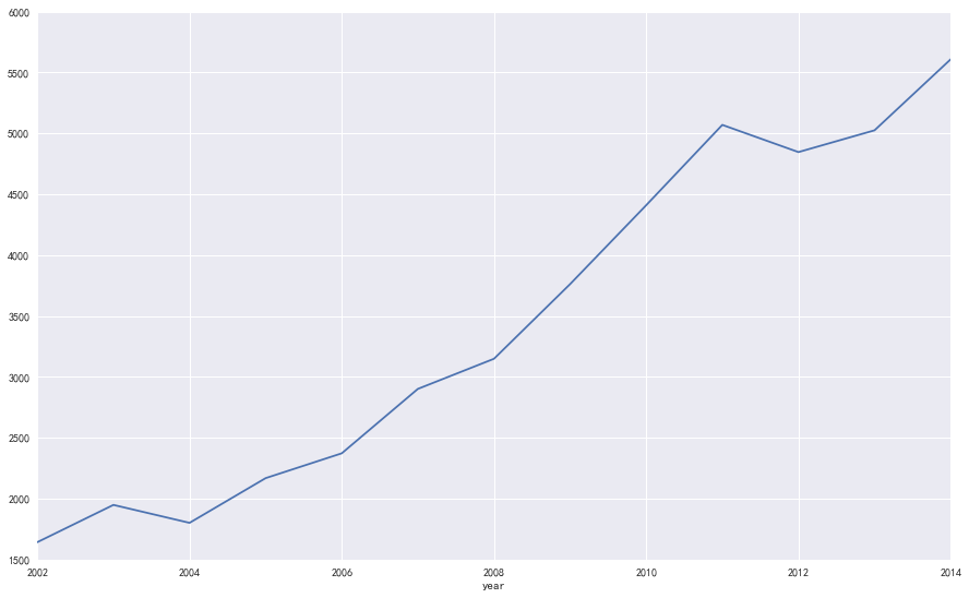
#获取贵阳数据集并绘图
gy = data['Guiyang']
print u'输出贵阳数据'
print gy
gy.plot()
plt.show()通过data['Guiyang']获取某列数据,然后再进行绘制如下所示:
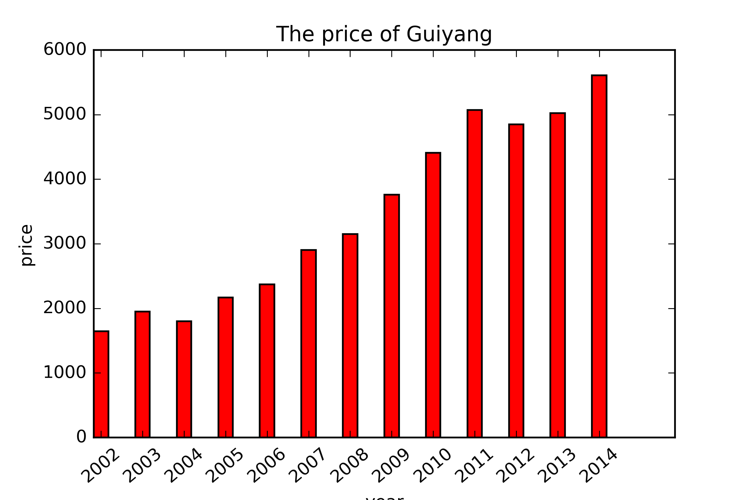
通过这个数据集调用bar函数可以绘制对应的柱状图,如下所示,需要注意x轴位年份,获取两列数据进行绘图。# -*- coding: utf-8 -*-
"""
Created on Mon Mar 06 10:55:17 2017
@author: eastmount
"""
import pandas as pd
data = pd.read_csv("32.csv",index_col='year') #index_col用作行索引的列名
#显示前6行数据
print(data.shape)
print(data.head(6))
#获取贵阳数据集并绘图
gy = data['Guiyang']
print u'输出贵阳数据'
print gy
import numpy as np
x = ['2002','2003','2004','2005','2006','2007','2008',
'2009','2010','2011','2012','2013','2014']
N = 13
ind = np.arange(N) #赋值0-13
width=0.35
plt.bar(ind, gy, width, color='r', label='sum num')
#设置底部名称
plt.xticks(ind+width/2, x, rotation=40) #旋转40度
plt.title('The price of Guiyang')
plt.xlabel('year')
plt.ylabel('price')
plt.savefig('guiyang.png',dpi=400)
plt.show()
输出如下图所示:
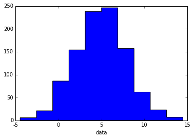
补充一段hist绘制柱状图的代码:import numpy as np
import pylab as pl
# make an array of random numbers with a gaussian distribution with
# mean = 5.0
# rms = 3.0
# number of points = 1000
data = np.random.normal(5.0, 3.0, 1000)
# make a histogram of the data array
pl.hist(data, histtype='stepfilled') #去掉黑色轮廓
# make plot labels
pl.xlabel('data')
pl.show()
输出如下图所示:
推荐文章:http://www.cnblogs.com/jasonfreak/p/5441512.html
时间序列相关文章推荐:
python时间序列分析
个股与指数的回归分析(python)
Python_Statsmodels包_时间序列分析_ARIMA模型
地址:http://www.dce.com.cn/dalianshangpin/xqsj/lssj/index.html#
比如下载"焦炭"数据集,命名为"35.csv",在对其进行聚类分析。
代码如下:
http://blog.csdn.net/xiaolewennofollow/article/details/46127485
代码如下:
# -*- coding: utf-8 -*-
"""
Created on Mon Mar 06 21:47:46 2017
@author: yxz
"""
from numpy import *
def loadDataSet(fileName,delim='\t'):
fr=open(fileName)
stringArr=[line.strip().split(delim) for line in fr.readlines()]
datArr=[map(float,line) for line in stringArr]
return mat(datArr)
def pca(dataMat,topNfeat=9999999):
meanVals=mean(dataMat,axis=0)
meanRemoved=dataMat-meanVals
covMat=cov(meanRemoved,rowvar=0)
eigVals,eigVets=linalg.eig(mat(covMat))
eigValInd=argsort(eigVals)
eigValInd=eigValInd[:-(topNfeat+1):-1]
redEigVects=eigVets[:,eigValInd]
print meanRemoved
print redEigVects
lowDDatMat=meanRemoved*redEigVects
reconMat=(lowDDatMat*redEigVects.T)+meanVals
return lowDDatMat,reconMat
dataMat=loadDataSet('41.txt')
lowDMat,reconMat=pca(dataMat,1)
def plotPCA(dataMat,reconMat):
import matplotlib
import matplotlib.pyplot as plt
datArr=array(dataMat)
reconArr=array(reconMat)
n1=shape(datArr)[0]
n2=shape(reconArr)[0]
xcord1=[];ycord1=[]
xcord2=[];ycord2=[]
for i in range(n1):
xcord1.append(datArr[i,0]);ycord1.append(datArr[i,1])
for i in range(n2):
xcord2.append(reconArr[i,0]);ycord2.append(reconArr[i,1])
fig=plt.figure()
ax=fig.add_subplot(111)
ax.scatter(xcord1,ycord1,s=90,c='red',marker='^')
ax.scatter(xcord2,ycord2,s=50,c='yellow',marker='o')
plt.title('PCA')
plt.savefig('ccc.png',dpi=400)
plt.show()
plotPCA(dataMat,reconMat)
输出结果如下图所示:
采用PCA方法对数据集进行降维操作,即将红色三角形数据降维至黄色直线上,一个平面降低成一条直线。PCA的本质就是对角化协方差矩阵,对一个n*n的对称矩阵进行分解,然后把矩阵投影到这N个基上。
数据集为41.txt,值如下:61.5 55
59.8 61
56.9 65
62.4 58
63.3 58
62.8 57
62.3 57
61.9 55
65.1 61
59.4 61
64 55
62.8 56
60.4 61
62.2 54
60.2 62
60.9 58
62 54
63.4 54
63.8 56
62.7 59
63.3 56
63.8 55
61 57
59.4 62
58.1 62
60.4 58
62.5 57
62.2 57
60.5 61
60.9 57
60 57
59.8 57
60.7 59
59.5 58
61.9 58
58.2 59
64.1 59
64 54
60.8 59
61.8 55
61.2 56
61.1 56
65.2 56
58.4 63
63.1 56
62.4 58
61.8 55
63.8 56
63.3 60
60.7 60
60.9 61
61.9 54
60.9 55
61.6 58
59.3 62
61 59
59.3 61
62.6 57
63 57
63.2 55
60.9 57
62.6 59
62.5 57
62.1 56
61.5 59
61.4 56
62 55.3
63.3 57
61.8 58
60.7 58
61.5 60
63.1 56
62.9 59
62.5 57
63.7 57
59.2 60
59.9 58
62.4 54
62.8 60
62.6 59
63.4 59
62.1 60
62.9 58
61.6 56
57.9 60
62.3 59
61.2 58
60.8 59
60.7 58
62.9 58
62.5 57
55.1 69
61.6 56
62.4 57
63.8 56
57.5 58
59.4 62
66.3 62
61.6 59
61.5 58
63.2 56
59.9 54
61.6 55
61.7 58
62.9 56
62.2 55
63 59
62.3 55
58.8 57
62 55
61.4 57
62.2 56
63 58
62.2 59
62.6 56
62.7 53
61.7 58
62.4 54
60.7 58
59.9 59
62.3 56
62.3 54
61.7 63
64.5 57
65.3 55
61.6 60
61.4 56
59.6 57
64.4 57
65.7 60
62 56
63.6 58
61.9 59
62.6 60
61.3 60
60.9 60
60.1 62
61.8 59
61.2 57
61.9 56
60.9 57
59.8 56
61.8 55
60 57
61.6 55
62.1 64
63.3 59
60.2 56
61.1 58
60.9 57
61.7 59
61.3 56
62.5 60
61.4 59
62.9 57
62.4 57
60.7 56
60.7 58
61.5 58
59.9 57
59.2 59
60.3 56
61.7 60
61.9 57
61.9 55
60.4 59
61 57
61.5 55
61.7 56
59.2 61
61.3 56
58 62
60.2 61
61.7 55
62.7 55
64.6 54
61.3 61
63.7 56.4
62.7 58
62.2 57
61.6 56
61.5 57
61.8 56
60.7 56
59.7 60.5
60.5 56
62.7 58
62.1 58
62.8 57
63.8 58
57.8 60
62.1 55
61.1 60
60 59
61.2 57
62.7 59
61 57
61 58
61.4 57
61.8 61
59.9 63
61.3 58
60.5 58
64.1 59
67.9 60
62.4 58
63.2 60
61.3 55
60.8 56
61.7 56
63.6 57
61.2 58
62.1 54
61.5 55
61.4 59
61.8 60
62.2 56
61.2 56
60.6 63
57.5 64
61.3 56
57.2 62
62.9 60
63.1 58
60.8 57
62.7 59
62.8 60
55.1 67
61.4 59
62.2 55
63 54
63.7 56
63.6 58
62 57
61.5 56
60.5 60
61.1 60
61.8 56
63.3 56
59.4 64
62.5 55
64.5 58
62.7 59
64.2 52
63.7 54
60.4 58
61.8 58
63.2 56
61.6 56
61.6 56
60.9 57
61 61
62.1 57
60.9 60
61.3 60
65.8 59
61.3 56
58.8 59
62.3 55
60.1 62
61.8 59
63.6 55.8
62.2 56
59.2 59
61.8 59
61.3 55
62.1 60
60.7 60
59.6 57
62.2 56
60.6 57
62.9 57
64.1 55
61.3 56
62.7 55
63.2 56
60.7 56
61.9 60
62.6 55
60.7 60
62 60
63 57
58 59
62.9 57
58.2 60
63.2 58
61.3 59
60.3 60
62.7 60
61.3 58
61.6 60
61.9 55
61.7 56
61.9 58
61.8 58
61.6 56
58.8 66
61 57
67.4 60
63.4 60
61.5 59
58 62
62.4 54
61.9 57
61.6 56
62.2 59
62.2 58
61.3 56
62.3 57
61.8 57
62.5 59
62.9 60
61.8 59
62.3 56
59 70
60.7 55
62.5 55
62.7 58
60.4 57
62.1 58
57.8 60
63.8 58
62.8 57
62.2 58
62.3 58
59.9 58
61.9 54
63 55
62.4 58
62.9 58
63.5 56
61.3 56
60.6 54
65.1 58
62.6 58
58 62
62.4 61
61.3 57
59.9 60
60.8 58
63.5 55
62.2 57
63.8 58
64 57
62.5 56
62.3 58
61.7 57
62.2 58
61.5 56
61 59
62.2 56
61.5 54
67.3 59
61.7 58
61.9 56
61.8 58
58.7 66
62.5 57
62.8 56
61.1 68
64 57
62.5 60
60.6 58
61.6 55
62.2 58
60 57
61.9 57
62.8 57
62 57
66.4 59
63.4 56
60.9 56
63.1 57
63.1 59
59.2 57
60.7 54
64.6 56
61.8 56
59.9 60
61.7 55
62.8 61
62.7 57
63.4 58
63.5 54
65.7 59
68.1 56
63 60
59.5 58
63.5 59
61.7 58
62.7 58
62.8 58
62.4 57
61 59
63.1 56
60.7 57
60.9 59
60.1 55
62.9 58
63.3 56
63.8 55
62.9 57
63.4 60
63.9 55
61.4 56
61.9 55
62.4 55
61.8 58
61.5 56
60.4 57
61.8 55
62 56
62.3 56
61.6 56
60.6 56
58.4 62
61.4 58
61.9 56
62 56
61.5 57
62.3 58
60.9 61
62.4 57
55 61
58.6 60
62 57
59.8 58
63.4 55
64.3 58
62.2 59
61.7 57
61.1 59
61.5 56
58.5 62
61.7 58
60.4 56
61.4 56
61.5 55
61.4 56
65 56
56 60
60.2 59
58.3 58
53.1 63
60.3 58
61.4 56
60.1 57
63.4 55
61.5 59
62.7 56
62.5 55
61.3 56
60.2 56
62.7 57
62.3 58
61.5 56
59.2 59
61.8 59
61.3 55
61.4 58
62.8 55
62.8 64
62.4 61
59.3 60
63 60
61.3 60
59.3 62
61 57
62.9 57
59.6 57
61.8 60
62.7 57
65.3 62
63.8 58
62.3 56
59.7 63
64.3 60
62.9 58
62 57
61.6 59
61.9 55
61.3 58
63.6 57
59.6 61
62.2 59
61.7 55
63.2 58
60.8 60
60.3 59
60.9 60
62.4 59
60.2 60
62 55
60.8 57
62.1 55
62.7 60
61.3 58
60.2 60
60.7 56
最后希望这篇文章对你有所帮助,尤其是我的学生和接触数据挖掘、机器学习的博友。这篇文字主要是记录一些代码片段,作为在线笔记,也希望对你有所帮助。
一醉一轻舞,一梦一轮回。一曲一人生,一世一心愿。
(By:Eastmount 2017-03-07 下午3点半 http://blog.csdn.net/eastmount/ )
如果文章中存在错误或不足之处,还请海涵~希望文章对你有所帮助。
一. Pandas获取数据集并显示
采用Pandas对2002年~2014年的商品房价数据集作时间序列分析,从中抽取几个城市与贵阳做对比,并对贵阳商品房作出分析。数据集位32.csv,具体值如下:(读者可直接复制)
year Beijing Chongqing Shenzhen Guiyang Kunming Shanghai Wuhai Changsha
2002 4764.00 1556.00 5802.00 1643.00 2276.00 4134.00 1928.00 1802.00
2003 4737.00 1596.00 6256.00 1949.00 2233.00 5118.00 2072.00 2040.00
2004 5020.93 1766.24 6756.24 1801.68 2473.78 5855.00 2516.32 2039.09
2005 6788.09 2134.99 7582.27 2168.90 2639.72 6842.00 3061.77 2313.73
2006 8279.51 2269.21 9385.34 2372.66 2903.32 7196.00 3689.64 2644.15
2007 11553.26 2722.58 14049.69 2901.63 3108.12 8361.00 4664.03 3304.74
2008 12418.00 2785.00 12665.00 3149.00 3750.00 8195.00 4781.00 3288.00
2009 13799.00 3442.00 14615.00 3762.00 3807.00 12840.00 5329.00 3648.00
2010 17782.00 4281.00 19170.00 4410.00 3660.00 14464.00 5746.00 4418.00
2011 16851.95 4733.84 21350.13 5069.52 4715.23 14603.24 7192.90 5862.39
2012 17021.63 5079.93 19589.82 4846.14 5744.68 14061.37 7344.05 6100.87
2013 18553.00 5569.00 24402.00 5025.00 5795.00 16420.00 7717.00 6292.00
2014 18833.00 5519.00 24723.00 5608.00 6384.00 16787.00 7951.00 6116.00
绘制对比各个城市的商品房价数据代码如下所示:
# -*- coding: utf-8 -*-
"""
Created on Mon Mar 06 10:55:17 2017
@author: eastmount
"""
import pandas as pd
data = pd.read_csv("32.csv",index_col='year') #index_col用作行索引的列名
#显示前6行数据
print(data.shape)
print(data.head(6))
import matplotlib.pyplot as plt
plt.rcParams['font.sans-serif'] = ['simHei'] #用来正常显示中文标签
plt.rcParams['axes.unicode_minus'] = False #用来正常显示负号
data.plot()
plt.savefig(u'时序图.png', dpi=500)
plt.show()
输出如下所示:
重点知识:
1、plt.rcParams显示中文及负号;
2、plt.savefig保存图片至本地;
3、pandas直接读取数据显示绘制图形,index_col获取索引。
二. Pandas获取某列数据绘制柱状图
接着上面的实验,我们需要获取贵阳那列数据,再绘制相关图形。# -*- coding: utf-8 -*-
"""
Created on Mon Mar 06 10:55:17 2017
@author: eastmount
"""
import pandas as pd
data = pd.read_csv("32.csv",index_col='year') #index_col用作行索引的列名
#显示前6行数据
print(data.shape)
print(data.head(6))
import matplotlib.pyplot as plt
plt.rcParams['font.sans-serif'] = ['simHei'] #用来正常显示中文标签
plt.rcParams['axes.unicode_minus'] = False #用来正常显示负号
data.plot()
plt.savefig(u'时序图.png', dpi=500)
plt.show()
#获取贵阳数据集并绘图
gy = data['Guiyang']
print u'输出贵阳数据'
print gy
gy.plot()
plt.show()通过data['Guiyang']获取某列数据,然后再进行绘制如下所示:
通过这个数据集调用bar函数可以绘制对应的柱状图,如下所示,需要注意x轴位年份,获取两列数据进行绘图。# -*- coding: utf-8 -*-
"""
Created on Mon Mar 06 10:55:17 2017
@author: eastmount
"""
import pandas as pd
data = pd.read_csv("32.csv",index_col='year') #index_col用作行索引的列名
#显示前6行数据
print(data.shape)
print(data.head(6))
#获取贵阳数据集并绘图
gy = data['Guiyang']
print u'输出贵阳数据'
print gy
import numpy as np
x = ['2002','2003','2004','2005','2006','2007','2008',
'2009','2010','2011','2012','2013','2014']
N = 13
ind = np.arange(N) #赋值0-13
width=0.35
plt.bar(ind, gy, width, color='r', label='sum num')
#设置底部名称
plt.xticks(ind+width/2, x, rotation=40) #旋转40度
plt.title('The price of Guiyang')
plt.xlabel('year')
plt.ylabel('price')
plt.savefig('guiyang.png',dpi=400)
plt.show()
输出如下图所示:
补充一段hist绘制柱状图的代码:import numpy as np
import pylab as pl
# make an array of random numbers with a gaussian distribution with
# mean = 5.0
# rms = 3.0
# number of points = 1000
data = np.random.normal(5.0, 3.0, 1000)
# make a histogram of the data array
pl.hist(data, histtype='stepfilled') #去掉黑色轮廓
# make plot labels
pl.xlabel('data')
pl.show()
输出如下图所示:
推荐文章:http://www.cnblogs.com/jasonfreak/p/5441512.html
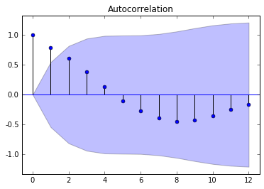
三. Python绘制时间序列-自相关图
核心代码如下所示:# -*- coding: utf-8 -*-
"""
Created on Mon Mar 06 10:55:17 2017
@author: yxz15
"""
import pandas as pd
data = pd.read_csv("32.csv",index_col='year')
#显示前6行数据
print(data.shape)
print(data.head(6))
import matplotlib.pyplot as plt
plt.rcParams['font.sans-serif'] = ['simHei']
plt.rcParams['axes.unicode_minus'] = False
data.plot()
plt.savefig(u'时序图.png', dpi=500)
plt.show()
from statsmodels.graphics.tsaplots import plot_acf
gy = data['Guiyang']
print gy
plot_acf(gy).show()
plt.savefig(u'贵阳自相关图',dpi=300)
from statsmodels.tsa.stattools import adfuller as ADF
print 'ADF:',ADF(gy)输出结果如下所示:时间序列相关文章推荐:
python时间序列分析
个股与指数的回归分析(python)
Python_Statsmodels包_时间序列分析_ARIMA模型
四. 聚类分析大连交易所数据集
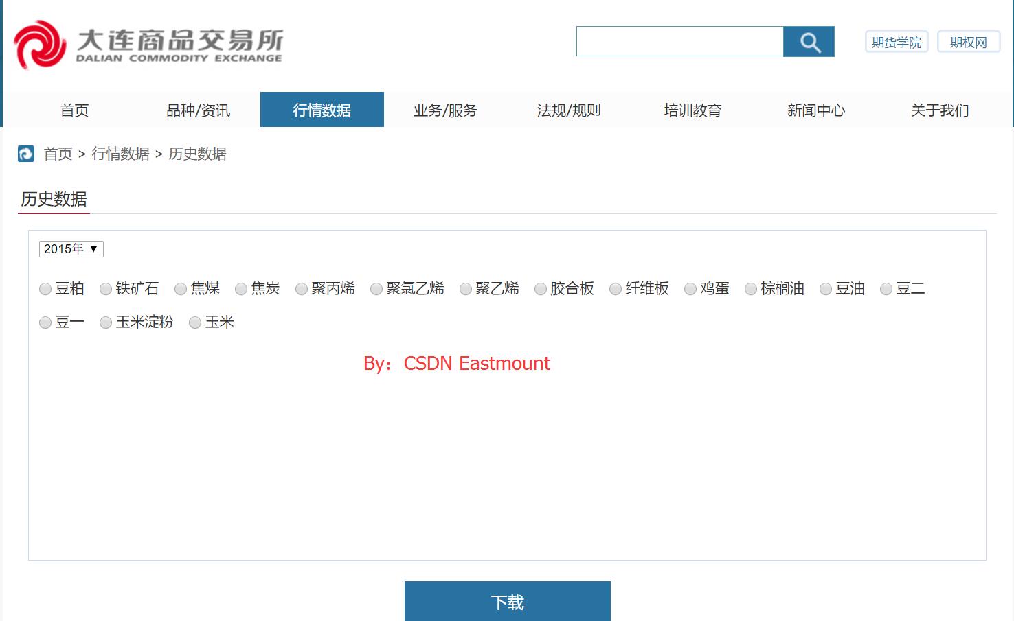
这部分主要提供一个网址给大家下载数据集,前面文章说过sklearn自带一些数据集以及UCI官网提供大量的数据集。这里讲述一个大连商品交易所的数据集。地址:http://www.dce.com.cn/dalianshangpin/xqsj/lssj/index.html#
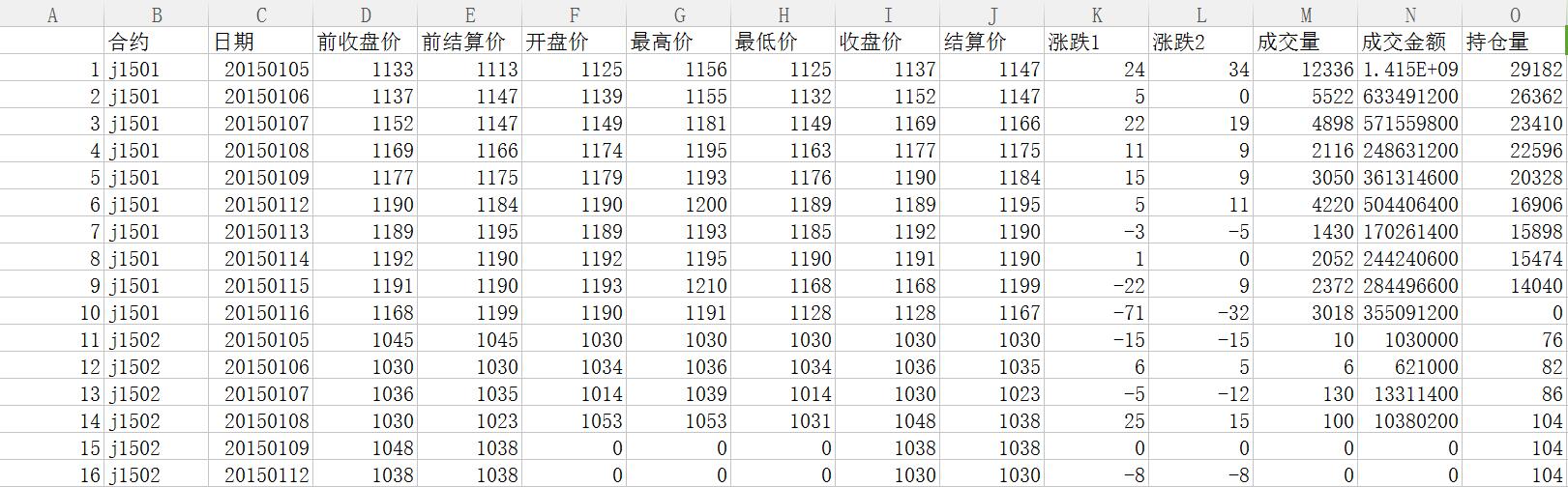
比如下载"焦炭"数据集,命名为"35.csv",在对其进行聚类分析。
代码如下:
# -*- coding: utf-8 -*-
"""
Created on Mon Mar 06 10:19:15 2017
@author: yxz15
"""
#第一部分:导入数据集
import pandas as pd
Coke1 =pd.read_csv("35.csv")
print Coke1 [:4]
#第二部分:聚类
from sklearn.cluster import KMeans
clf=KMeans(n_clusters=3)
pre=clf.fit_predict(Coke1)
print pre[:4]
#第三部分:降维
from sklearn.decomposition import PCA
pca=PCA(n_components=2)
newData=pca.fit_transform(Coke1)
print newData[:4]
x1=[n[0] for n in newData]
x2=[n[1] for n in newData]
#第四部分:用matplotlib包画图
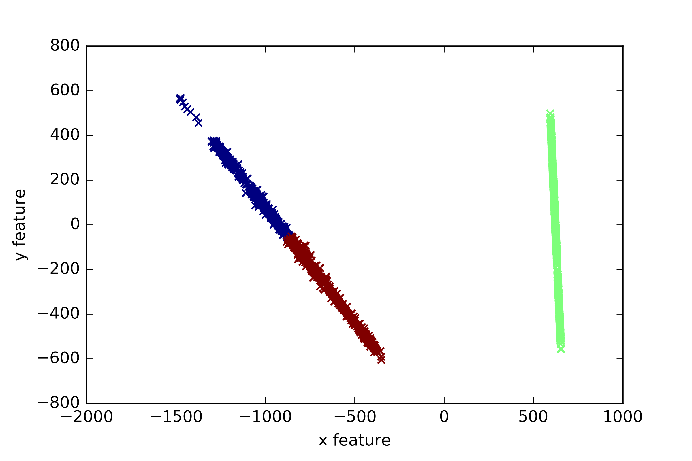
import matplotlib.pyplot as plt
plt.title
plt.xlabel("x feature")
plt.ylabel("y feature")
plt.scatter(x1,x2,c=pre, marker='x')
plt.savefig("bankloan.png",dpi=400)
plt.show()输出如下图所示:五. PCA降维及绘图代码
PCA降维绘图参考这篇博客。http://blog.csdn.net/xiaolewennofollow/article/details/46127485
代码如下:
# -*- coding: utf-8 -*-
"""
Created on Mon Mar 06 21:47:46 2017
@author: yxz
"""
from numpy import *
def loadDataSet(fileName,delim='\t'):
fr=open(fileName)
stringArr=[line.strip().split(delim) for line in fr.readlines()]
datArr=[map(float,line) for line in stringArr]
return mat(datArr)
def pca(dataMat,topNfeat=9999999):
meanVals=mean(dataMat,axis=0)
meanRemoved=dataMat-meanVals
covMat=cov(meanRemoved,rowvar=0)
eigVals,eigVets=linalg.eig(mat(covMat))
eigValInd=argsort(eigVals)
eigValInd=eigValInd[:-(topNfeat+1):-1]
redEigVects=eigVets[:,eigValInd]
print meanRemoved
print redEigVects
lowDDatMat=meanRemoved*redEigVects
reconMat=(lowDDatMat*redEigVects.T)+meanVals
return lowDDatMat,reconMat
dataMat=loadDataSet('41.txt')
lowDMat,reconMat=pca(dataMat,1)
def plotPCA(dataMat,reconMat):
import matplotlib
import matplotlib.pyplot as plt
datArr=array(dataMat)
reconArr=array(reconMat)
n1=shape(datArr)[0]
n2=shape(reconArr)[0]
xcord1=[];ycord1=[]
xcord2=[];ycord2=[]
for i in range(n1):
xcord1.append(datArr[i,0]);ycord1.append(datArr[i,1])
for i in range(n2):
xcord2.append(reconArr[i,0]);ycord2.append(reconArr[i,1])
fig=plt.figure()
ax=fig.add_subplot(111)
ax.scatter(xcord1,ycord1,s=90,c='red',marker='^')
ax.scatter(xcord2,ycord2,s=50,c='yellow',marker='o')
plt.title('PCA')
plt.savefig('ccc.png',dpi=400)
plt.show()
plotPCA(dataMat,reconMat)
输出结果如下图所示:
采用PCA方法对数据集进行降维操作,即将红色三角形数据降维至黄色直线上,一个平面降低成一条直线。PCA的本质就是对角化协方差矩阵,对一个n*n的对称矩阵进行分解,然后把矩阵投影到这N个基上。
数据集为41.txt,值如下:61.5 55
59.8 61
56.9 65
62.4 58
63.3 58
62.8 57
62.3 57
61.9 55
65.1 61
59.4 61
64 55
62.8 56
60.4 61
62.2 54
60.2 62
60.9 58
62 54
63.4 54
63.8 56
62.7 59
63.3 56
63.8 55
61 57
59.4 62
58.1 62
60.4 58
62.5 57
62.2 57
60.5 61
60.9 57
60 57
59.8 57
60.7 59
59.5 58
61.9 58
58.2 59
64.1 59
64 54
60.8 59
61.8 55
61.2 56
61.1 56
65.2 56
58.4 63
63.1 56
62.4 58
61.8 55
63.8 56
63.3 60
60.7 60
60.9 61
61.9 54
60.9 55
61.6 58
59.3 62
61 59
59.3 61
62.6 57
63 57
63.2 55
60.9 57
62.6 59
62.5 57
62.1 56
61.5 59
61.4 56
62 55.3
63.3 57
61.8 58
60.7 58
61.5 60
63.1 56
62.9 59
62.5 57
63.7 57
59.2 60
59.9 58
62.4 54
62.8 60
62.6 59
63.4 59
62.1 60
62.9 58
61.6 56
57.9 60
62.3 59
61.2 58
60.8 59
60.7 58
62.9 58
62.5 57
55.1 69
61.6 56
62.4 57
63.8 56
57.5 58
59.4 62
66.3 62
61.6 59
61.5 58
63.2 56
59.9 54
61.6 55
61.7 58
62.9 56
62.2 55
63 59
62.3 55
58.8 57
62 55
61.4 57
62.2 56
63 58
62.2 59
62.6 56
62.7 53
61.7 58
62.4 54
60.7 58
59.9 59
62.3 56
62.3 54
61.7 63
64.5 57
65.3 55
61.6 60
61.4 56
59.6 57
64.4 57
65.7 60
62 56
63.6 58
61.9 59
62.6 60
61.3 60
60.9 60
60.1 62
61.8 59
61.2 57
61.9 56
60.9 57
59.8 56
61.8 55
60 57
61.6 55
62.1 64
63.3 59
60.2 56
61.1 58
60.9 57
61.7 59
61.3 56
62.5 60
61.4 59
62.9 57
62.4 57
60.7 56
60.7 58
61.5 58
59.9 57
59.2 59
60.3 56
61.7 60
61.9 57
61.9 55
60.4 59
61 57
61.5 55
61.7 56
59.2 61
61.3 56
58 62
60.2 61
61.7 55
62.7 55
64.6 54
61.3 61
63.7 56.4
62.7 58
62.2 57
61.6 56
61.5 57
61.8 56
60.7 56
59.7 60.5
60.5 56
62.7 58
62.1 58
62.8 57
63.8 58
57.8 60
62.1 55
61.1 60
60 59
61.2 57
62.7 59
61 57
61 58
61.4 57
61.8 61
59.9 63
61.3 58
60.5 58
64.1 59
67.9 60
62.4 58
63.2 60
61.3 55
60.8 56
61.7 56
63.6 57
61.2 58
62.1 54
61.5 55
61.4 59
61.8 60
62.2 56
61.2 56
60.6 63
57.5 64
61.3 56
57.2 62
62.9 60
63.1 58
60.8 57
62.7 59
62.8 60
55.1 67
61.4 59
62.2 55
63 54
63.7 56
63.6 58
62 57
61.5 56
60.5 60
61.1 60
61.8 56
63.3 56
59.4 64
62.5 55
64.5 58
62.7 59
64.2 52
63.7 54
60.4 58
61.8 58
63.2 56
61.6 56
61.6 56
60.9 57
61 61
62.1 57
60.9 60
61.3 60
65.8 59
61.3 56
58.8 59
62.3 55
60.1 62
61.8 59
63.6 55.8
62.2 56
59.2 59
61.8 59
61.3 55
62.1 60
60.7 60
59.6 57
62.2 56
60.6 57
62.9 57
64.1 55
61.3 56
62.7 55
63.2 56
60.7 56
61.9 60
62.6 55
60.7 60
62 60
63 57
58 59
62.9 57
58.2 60
63.2 58
61.3 59
60.3 60
62.7 60
61.3 58
61.6 60
61.9 55
61.7 56
61.9 58
61.8 58
61.6 56
58.8 66
61 57
67.4 60
63.4 60
61.5 59
58 62
62.4 54
61.9 57
61.6 56
62.2 59
62.2 58
61.3 56
62.3 57
61.8 57
62.5 59
62.9 60
61.8 59
62.3 56
59 70
60.7 55
62.5 55
62.7 58
60.4 57
62.1 58
57.8 60
63.8 58
62.8 57
62.2 58
62.3 58
59.9 58
61.9 54
63 55
62.4 58
62.9 58
63.5 56
61.3 56
60.6 54
65.1 58
62.6 58
58 62
62.4 61
61.3 57
59.9 60
60.8 58
63.5 55
62.2 57
63.8 58
64 57
62.5 56
62.3 58
61.7 57
62.2 58
61.5 56
61 59
62.2 56
61.5 54
67.3 59
61.7 58
61.9 56
61.8 58
58.7 66
62.5 57
62.8 56
61.1 68
64 57
62.5 60
60.6 58
61.6 55
62.2 58
60 57
61.9 57
62.8 57
62 57
66.4 59
63.4 56
60.9 56
63.1 57
63.1 59
59.2 57
60.7 54
64.6 56
61.8 56
59.9 60
61.7 55
62.8 61
62.7 57
63.4 58
63.5 54
65.7 59
68.1 56
63 60
59.5 58
63.5 59
61.7 58
62.7 58
62.8 58
62.4 57
61 59
63.1 56
60.7 57
60.9 59
60.1 55
62.9 58
63.3 56
63.8 55
62.9 57
63.4 60
63.9 55
61.4 56
61.9 55
62.4 55
61.8 58
61.5 56
60.4 57
61.8 55
62 56
62.3 56
61.6 56
60.6 56
58.4 62
61.4 58
61.9 56
62 56
61.5 57
62.3 58
60.9 61
62.4 57
55 61
58.6 60
62 57
59.8 58
63.4 55
64.3 58
62.2 59
61.7 57
61.1 59
61.5 56
58.5 62
61.7 58
60.4 56
61.4 56
61.5 55
61.4 56
65 56
56 60
60.2 59
58.3 58
53.1 63
60.3 58
61.4 56
60.1 57
63.4 55
61.5 59
62.7 56
62.5 55
61.3 56
60.2 56
62.7 57
62.3 58
61.5 56
59.2 59
61.8 59
61.3 55
61.4 58
62.8 55
62.8 64
62.4 61
59.3 60
63 60
61.3 60
59.3 62
61 57
62.9 57
59.6 57
61.8 60
62.7 57
65.3 62
63.8 58
62.3 56
59.7 63
64.3 60
62.9 58
62 57
61.6 59
61.9 55
61.3 58
63.6 57
59.6 61
62.2 59
61.7 55
63.2 58
60.8 60
60.3 59
60.9 60
62.4 59
60.2 60
62 55
60.8 57
62.1 55
62.7 60
61.3 58
60.2 60
60.7 56
最后希望这篇文章对你有所帮助,尤其是我的学生和接触数据挖掘、机器学习的博友。这篇文字主要是记录一些代码片段,作为在线笔记,也希望对你有所帮助。
一醉一轻舞,一梦一轮回。一曲一人生,一世一心愿。
(By:Eastmount 2017-03-07 下午3点半 http://blog.csdn.net/eastmount/ )

相关文章推荐
- python数据挖掘课程 十.Pandas、Matplotlib、PCA绘图实用代码补充
- 【python数据挖掘课程】十.Pandas、Matplotlib、PCA绘图实用代码补充
- python数据挖掘学习笔记】十.Pandas、Matplotlib、PCA绘图实用代码补充
- 【python数据挖掘课程】十二.Pandas、Matplotlib结合SQL语句对比图分析
- 【python数据挖掘课程】十二.Pandas、Matplotlib结合SQL语句对比图分析
- 【python数据挖掘课程】十一.Pandas、Matplotlib结合SQL语句可视化分析
- python数据挖掘课程 十二.Pandas、Matplotlib结合SQL语句对比图分析
- python数据挖掘课程 十一.Pandas、Matplotlib结合SQL语句可视化分析
- 【python数据挖掘课程】十一.Pandas、Matplotlib结合SQL语句可视化分析
- python 实现将 pandas 数据和 matplotlib 绘图嵌入 html 文件
- Python数据分析与挖掘实战(Pandas,Matplotlib常用方法)
- python绘图:matplotlib和pandas的应用
- python数据分析学习笔记-Numpy-Matplotlib-Pandas
- python:matplotlib及pandas绘图(1)
- Python数据可视化利器Matplotlib,绘图入门篇,Pyplot介绍
- python数据分析之(6)简单绘图matplotlib.pyplot
- 基于Python的数据可视化 matplotlib seaborn pandas
- Python进阶(三十九)-数据可视化の使用matplotlib进行绘图分析数据
- 获取博客积分排名,存入数据库,读取数据进行绘图(python,selenium,matplotlib)
- python3.6中安装numpy,pandas,scipy,scikit_learn,matplotlib等数据分析工具