单因素特征选择--Univariate Feature Selection

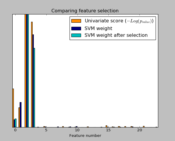
An example showing univariate feature selection.

Noisy (non informative) features are added to the iris data and univariate feature selection（单因素特征选择） is applied. For each feature, we plot the p-values for the univariate feature selection and the corresponding weights of an SVM. We can see that univariate feature selection selects the informative features and that these have larger SVM weights.

In the total set of features, only the 4 first ones are significant. We can see that they have the highest score with univariate feature selection. The SVM assigns a large weight to one of these features, but also Selects many of the non-informative features. Applying univariate feature selection before the SVM increases the SVM weight attributed to the significant features, and will thus improve classification.

#encoding:utf-8
import numpy as np
import matplotlib.pyplot as plt
from sklearn import datasets,svm
from sklearn.feature_selection import SelectPercentile,f_classif

###load iris dateset
iris=datasets.load_iris()

###Some Noisy data not correlated
E=np.random.uniform(0,0.1,size=(len(iris.data),20)) ###uniform distribution   150*20
X=np.hstack((iris.data,E))
y=iris.target

plt.figure(1)
plt.clf()

X_indices=np.arange(X.shape[-1])   ###X.shape=(150,24)    X.shape([-1])=24

selector=SelectPercentile(f_classif,percentile=10)
selector.fit(X,y)
scores=-np.log10(selector.pvalues_)
scores/=scores.max()

plt.bar(X_indices-0.45,scores,width=0.2,label=r"Univariate score ($-Log(p_{value})$)",color='darkorange')
# plt.show()

####Compare to weight of an svm
clf=svm.SVC(kernel='linear')
clf.fit(X,y)

svm_weights=(clf.coef_**2).sum(axis=0)
svm_weights/=svm_weights.max()
plt.bar(X_indices - .25, svm_weights, width=.2, label='SVM weight',
color='navy')
clf_selected=svm.SVC(kernel='linear')
# clf_selected.fit(selector.transform((X,y)))
clf_selected.fit(selector.transform(X),y)

svm_weights_selected=(clf_selected.coef_**2).sum(axis=0)
svm_weights_selected/=svm_weights_selected.max()

plt.bar(X_indices[selector.get_support()]-.05,svm_weights_selected,width=.2,label='SVM weight after selection',color='c')

plt.title("Comparing feature selection")
plt.xlabel('Feature number')
plt.yticks(())
plt.axis('tight')
plt.legend(loc='upper right')
plt.show()

实验结果：