CS231n-线性SVM分类Cifar10

线性SVM
目标函数

代价函数
正则项

梯度计算

向量化构建SVM模型
train函数
小批量梯度下降

计算代价函数和梯度值

梯度下降

predict函数

使用SVM模型分类CIFAR10
数据预处理

自动化确定超参

通过参数和训练集来构建模型并预测测试集准确率

完整代码

线性分类器其实我已经接触不少了，不同于KNN，它涉及到了更多的知识，比如cost function, objective function等，svm涉及到的知识确实比较多且难理解，但当我们得到相应公式后其实实现起来并不算繁琐，相反很容易理解

线性SVM

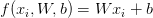
目标函数

目标函数我们在以前的线性回归，逻辑回归中都见到过

代价函数

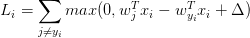
SVM的代价函数想要SVM在正确分类上的得分始终比不正确分类上的得分高出一个边界值delta, 所以它的代价函数如下：



即在确定正确分类的分数（scores[y[i]]）后，其他分类上的分数都要减去它并且加上一个边界值 ( scores[y[!i] - screos[y[i]] + delta )，当得到的值小于0时则代表正确分类比不正确分类高出了一个边界值，否则则要计算损失值。 比如，假设有3个分类，并且得到了分值[13, -7, 11], 第一个分类为正确分类，delta为10，那么根据代价函数，我们可以得到以下算式



以上代价函数计算公式称为折叶损失（hinge loss），当然除此之外还有平方折叶损失SVM（即L2-SVM），就是加个平方，我们可以通过交叉验证或者验证集来确定到底选用哪个

正则项

在ML中，过拟合问题一直是影响模型准确率的重大因素，所以我们还要加上L2范式正则项（在这里，正则项还确保了SVM有最大边界（max margin）等好处），所以最终我们得到以下整个代价函数公式

梯度计算

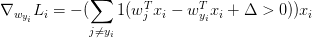
在训练过程中，我们需要通过最优化方法来是代价函数的损失值达到尽可能的小，所以我们对代价函数进行微分，然后计算其偏导数，得到以下公式

对于每一个训练样本，我们计算它在每个分类上的得分，每当它在某一分类产生了损失（即scores[y[!i] - screos[y[i]] + delta > 0），那么我们就将该分类上的参数梯度+Xi



同时正确分类（y[i]）的参数梯度-Xi



再简单的说就是，对于每个Xi，每一个会产生损失值的分类（scores[y[!i] - screos[y[i]] + delta > 0）都会将其参数梯度+Xi，同时在正确分类（y[i]）上的梯度-Xi

将以上的公式转化成代码，用非向量化实现（更容易理解）如下

def svm_loss_naive(W, X, y, reg):
"""
Structured SVM loss function, naive implementation (with loops).

Inputs have dimension D, there are C classes, and we operate on minibatches
of N examples.

Inputs:
- W: A numpy array of shape (D, C) containing weights.
- X: A numpy array of shape (N, D) containing a minibatch of data.
- y: A numpy array of shape (N,) containing training labels; y[i] = c means
that X[i] has label c, where 0 <= c < C.
- reg: (float) regularization strength

Returns a tuple of:
- loss as single float
- gradient with respect to weights W; an array of same shape as W
"""
dW = np.zeros(W.shape) # initialize the gradient as zero

# compute the loss and the gradient
num_classes = W.shape[1]
num_train = X.shape[0]
loss = 0.0
for i in range(num_train):
scores = X[i].dot(W)
correct_class_score = scores[y[i]]
for j in range(num_classes):
if j == y[i]:
continue
margin = scores[j] - correct_class_score + 1 # note delta = 1
if margin > 0:
loss += margin

# cal gred
dW[:, j] += X[i]
dW[:, y[i]] -= X[i]

# Right now the loss is a sum over all training examples, but we want it
# to be an average instead so we divide by num_train.
loss /= num_train
dW /= num_train

# Add regularization to the loss.
loss += 0.5 * reg * np.sum(W * W)
dW += reg * W

return loss, dW

向量化构建SVM模型

非向量化的实现易于理解，但是我们在实际使用时当然要考虑效率问题，所以接下来我们使用向量化的方式该模型，模型包括train和predict函数

train函数

train函数包括计算代价函数和梯度值，同时运用梯度下降来得到最终的参数W

小批量梯度下降

由于CIFAR10数据集比较大，如果我们使用批量梯度下降的方法效率很低，所以我们这里使用小批量梯度下降

# Mini-batch 每次迭代时随机取batch_num个作为训练集
sample_index = np.random.choice(num_train, batch_num, replace=False)
X_batch = X[sample_index, :]
y_batch = y[sample_index]

计算代价函数和梯度值

这里由于要实际应用，所以非向量化的实现效率太低，这里采用向量化实现方法，主要用到了numpy库

def svm_cost_function(self, X, y, reg, delta):
""" cal loss

:param X: A numpy array of shape (N, D)
:param y: A numpy array of shape (N, )
:param reg: regularization strength
:param delta: margin
:return: loss, gred
"""
num_train = X.shape[0]

scores = X.dot(self.W.T)  # N * C
correct_class_scores = scores[range(num_train), y]
margins = scores - correct_class_scores[:, np.newaxis] + delta
margins = np.maximum(0, margins)
# do not ignore it, because 'y - y + delta' > 0, we should reset it to zeros
margins[range(num_train), y] = 0

loss = np.sum(margins) / num_train + 0.5 * reg * np.sum(self.W * self.W)

# cal gred [for every example, when margin > 0, correct lable's W should -X, and wrong lable's W should +X]
ground_true = np.zeros(margins.shape)  # N * C
ground_true[margins > 0] = 1
sum_margins = np.sum(ground_true, axis=1)
ground_true[range(num_train), y] -= sum_margins

gred = ground_true.T.dot(X) / num_train + reg * self.W

return loss, gred

梯度下降

这里使用SGD（指mini-batch gradient descent）实现梯度下降，学习率的确定可以通过验证集或交叉验证来确定

loss, gred = self.svm_cost_function(X_batch, y_batch, reg, delta)
self.W -= learning_rate * gred

predict函数

在训练完之后，模型的参数就已经确定了，所以预测是非常简单的，只需要将每个测试集的X对每个分类计算分数，并将分数最高的作为分类

def predict(self, X):
""" predict

:param X: A numpy array of shape (N, D)
:return: y_pred (A numpy array of shape (N, ))
"""
scores = X.dot(self.W.T)

y_pred = np.zeros(X.shape[0])
y_pred = np.argmax(scores, axis=1)

return y_pred

使用SVM模型分类CIFAR10

数据预处理

对于读取进来的cifar10数据，我们首先要做一些必要的预处理，即对每个特征减去平均值来中心化数据，这样图像的像素值就大约分布在[-127, 127]之间，当然我们还可以让所有数值分布的区间变为[-1, 1]，同时将数据分为训练集，测试集和验证集，分别用于训练，测试和确定超参

自动化确定超参

原理非常简单，对每一组参数分别使用训练集训练模型，然后用验证集来得到分类准确率来比较其泛化能力从而选出最优的参数

for i in learning_rates:
for j in regularization_strengths:
svm = SVM()
# X, y, reg, delta, learning_rate, batch_num, num_iter, debug
svm.train(X_train, y_train, j, 1, i, 200, 1500, True)
y_pred = svm.predict(X_val)
acc_val = np.mean(y_val == y_pred)
if best_val < acc_val:
best_val = acc_val
best_parameter = (i, j)

通过参数和训练集来构建模型并预测测试集准确率

在这一步就是简单的调用模型函数即可，如果你记录下了loss，那么我们还可以可视化loss的走向趋势图



测试集的最终结果准确率大概在37%左右

完整代码

CS231n的代码均保存到了 github/cs231n 上