【Caffe安装】caffe安装系列——史上最详细的安装步骤
2016-11-21 15:10
459 查看
说明
网上关于caffe的安装教程非常多,但是关于每一步是否操作成功,出现了什么样的错误又该如何处理没有给出说明。因为大家的操作系统的环境千差万别,按照博客中的教程一步步的安装,最后可能失败——这是很常见的哦。有的教程甚至省略了一些细节部分,让小白更不知道如何判断每一步是否操作成功,如何处理出现的错误。作者花费了很长时间才成功地将caffe装完,期间遇到好多错误,多次重装操作系统。现在将经验写下来,一方面为了和大家分享,讨论;另一方面是为了记录一下下~~~
环境
操作系统:Ubuntu 14.04GCC/G++:4.7.x
OpenCV:2.4.11和3.0.0
Matlab :R2014b(a)
Python:2.7
安装步骤
综述0.准备工作
1.安装GCC4.7和G++4.7并降级
2.安装显卡驱动
3.安装cuda和cudnn
4.安装Matlab
5.安装OpenCV
6.安装Python依赖包
7.安装caffe
介绍
0.准备工作
安装Ubuntu 14.04(15.04),最好安装较新版本的Ubuntu。为什么选择Ubuntu呢?一方面,个人使用习惯,感觉Ubuntu安装软件等特别方便,使用特别顺手;另一方面,caffe项目最初貌似在Ubuntu上开发的,原生嘛。安装过程需要下载东东,因此需要联网。
安装
1.安装GCC4.7和G++4.7并降级
为什么要先安装GCC和G++,并需要降级呢?Ubuntu14.04版本默认的GCC和G++都是4.8。而Matlab默认支持的mex编译器是GCC4.7.x和G++4.7.x。因此需要额外安装GCC4.7和G++4.7并降级。
为什么需要先安装编译器GCC和G++,而不是先安装显卡驱动和cuda等等呢?
首先,先安装显卡驱动,后安装GCC并降级的安装顺序过程中,遇到了很多问题。比如,在安装CUDA SAMPLES的过程中,遇到了问题/usr/bin/ld: cannot find –lGL,后面通过网上教程,重新连接该库文件,仍然不能通过OpenCV的编译。但是,先安装GCC,再安装显卡驱动,就不会遇到这个问题了。
其次,请先看下图。这是在成功地安装完显卡驱动之后,查看加载的显卡的版本信息时返回的结果。注意,包含了GCC4.7.3。说明,显卡安装过程中,会和GCC的版本产生联系。。。。这也就不不难理解为什么在编译Cuda Samples过程中会遇到上面的问题。
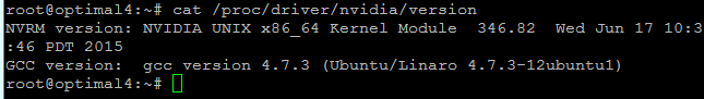
所以,请先安装GCC4.7和G++4.7,然后在执行下面的步骤。
2.安装NVIDIA显卡驱动
为什么需要安装NVIDIA显卡驱动,Ubuntu没有自带的显卡驱动吗?Ubuntu自带的显卡驱动是开源的Nouveau,据说是一个比较烂的东东。而且,最关键的是cuda不支持Nouveau。如果想使用cuda进行GPU计算,必须安装NVIDIA显卡驱动。
选择哪个版本的显卡驱动呢
这个问题需要结合操作系统,显卡和个人需求来讨论。
操作系统影响显卡驱动的版本。比如,我在Ubuntu14.04 Server上安装NVIDIA-352显卡驱动,说是由于dkms,安装失败。目前,通过apt-get方式可以安装的最新NVIDIA显卡驱动是NVIDIA-346。
显卡嘛,硬件当然要和驱动适应才行
个人需求,主要从cuda的角度考虑。比如cuda7.5需要显卡驱动最低版本是nvidia-352;cuda7.0需要显卡驱动最低版本是nvidia-336;cuda6.5需要显卡驱动最低版本是nvidia-33*;其他的记不清楚啦。。。
显卡驱动的安装方式有哪些
方法一:去NVIDIA官网下载相应的驱动二进制安装包,然后安装。
方法二:通过
apt-get来安装。
区别:apt-get安装方便,但是不能安装最新的显卡驱动,目前ubuntu14.04通过apt-get可以安装nvidia-346显卡。
安装过程中注意事项:①需要关闭显示管理器,②二进制安装需要修改文件,并重启。
3.安装cuda和cudnn
安装cuda的方式有哪些?方法一:官网下载cuda开发包的二进制安装包进行安装。
方法二:官网下载cuda开发包的deb文件进行安装。
cuda版本的选择问题?
根据个人需求和操作系统来决定,显卡驱动版本。
cuda6.5是一个分界点,cuda6.5支持compute_11,compute_12. etc. compute_1X系列架构;从cuda7.0开始,不支持compute_1X系列架构,最低是compute_20架构。
cuda对显卡驱动有要求。比如cuda7.5需要显卡驱动最低版本是nvidia-352;cuda7.0需要显卡驱动最低版本是nvidia-336;cuda6.5需要显卡驱动最低版本是nvidia-33*;其他的记不清楚啦。因此,结合自己操作系统可以安装的NVIDIA显卡驱动来决定选择哪个版本的cuda。
为什么安装cudnn?
cudnn可以简单的理解为
CUDa cNN,即在GPU上做卷积运算。最近几年,深度学习很火,尤其是CNN(卷积神经网络)。通过cudnn,可以极大的提高CNN训练速度。简单的说,实用GPU是为了快,实用cudnn是为了更快。
4.安装Matlab
在Ubuntu中安装Matlab比较简单,除了几个注意事项,和Windows中安装没有区别。为什么需要安装Matlab?
caffe有Matlab的接口,因此如果需要使用Matlab调用caffe,进行编程,就需要安装Matlab。如果你觉得使用C或Python编程比较难,就请安装Matlab。当然如果不需要,并且后面不会编译caffe生成Matlab的接口,就不需要安装Matlab了。这个纯粹根据个人需求来定。
Matlab是商业软件,请自行百度下载。。。【主要是太大了,不方便提供】
5.安装OpenCV
为什么需要安装OpenCV?caffe是用来做深度学习的,深度学习的一大应用对象就是图像和视频。而OpenCV是目前最火的开源计算机视觉库,非常多的项目多用到了OpenCV,当然caffe也依赖OpenCV。所以,需要安装OpenCV,否则无法使用caffe哦。。。
OpenCV安装简单吗?
答案是因人而异。有的人觉得简单,可以自己弄,有的人觉得难,没关系,大神们有写的安装脚本点此*下载,运行一下就OK了。
但是,使用别人脚本安装的方法,也会遇到一些问题。如果遇到问题,请Google解决。
最简单的方式是使用我修改过的脚本,按照顺序执行12345个脚本,基本不需要修改就能成功安装。
最后提醒,安装OpenCV是挺麻烦的,请耐心安装,编译不过的话,查看错误Google,解决了再编译,一遍遍的尝试,最后就能解决问题了。
应该安装OpenCV哪个版本呢?
OpenCV的版本和cuda的版本最好匹配。这样子安排的目的是为了减少错误出现的概率。比如,我无错误编译成功的组合有【cuda7.0 + opencv3.0】,【cuda6.5+opencv2.11】。
应该安装最新的,又不该安装最新的。呵呵,好别扭哦。针对于低版本的cuda,最好安装opencv2.x。而且是opencv2.x中最新的。
低版本cuda安装opencv2.x的原因是,opencv的一些文件中涉及一些关于cuda架构的设置,opencv2.x中有支持相应的架构的配置。从这个角度看,cuda6.5是最保险的, 因为它既支持compute_1x,也支持更高的架构。
6.安装Python相关依赖
为什么要安装python相关依赖???首先,python在linux中应用非常的广泛,很多项目都会涉及python,caffe也不例外。
其次,caffe提供了python的接口,为了后面使用,也需要这些依赖。
这些依赖都可以通过apt-get安装吗?
答案是否定的。
首先,google一下
apt-get vs pip,查看两者区别。
其次,安装theano的时候,发现apt-get安装的numPy和sciPy无法通过测试,并且造成theano测试失败。使用pip安装成功。参考《Ubuntu14.04安装Theano详细教程》。
最后,在安装caffe的过程中,发现有几个python依赖包必须通过pip安装(即自行编译),否则无法成功地编译caffe。
6.安装caffe
再重复一遍,请在上面所有步骤成功执行的前提下,安装caffe,否则编译肯定不会通过的。caffe源代码能不能直接拿过来编译呢?
不能。至少需要修改一个文件Makefile.config。该文件给caffe编译提供了必要的信息。
如果opencv的版本是3.0,还需要修改其他项。
其他的请参考安装caffe的教程
总结
至此,ubuntu下安装caffe的工作已经结束了。如果你完全按照本教程操作,相信你一定已经成功安装caffe了,并且对caffe有了一定的了解。世上无难事只怕有坚持,安装过程虽然很复杂,但是只要坚持,不断的Google解决它,caffe就一定能安装。
错误不可怕,它是成功的障碍,同时也为我们成长提供了阶梯——所谓的能力,很大一部分是通过不断解决问题来获取的。
下面开始学习如何使用caffe做深度学习的研究喽,祝大家学习愉快。。。
参考
《Caffe + Ubuntu 15.04 + CUDA 7.0 新手安装配置指南》——欧新宇这个教程很好,请查看本教程的过程中,结合欧新宇的教程一并查看。
《caffe - GitHub主页》
网络结构在线可视化工具
http://ethereon.github.io/netscope/#/editor
参考主页:
caffe 可视化的资料可在百度云盘下载
链接: http://pan.baidu.com/s/1jIRJ6mU
提取密码:xehi
http://cs.stanford.edu/people/karpathy/cnnembed/
http://lijiancheng0614.github.io/2015/08/21/2015_08_21_CAFFE_Features/
http://nbviewer.ipython.org/github/BVLC/caffe/blob/master/examples/00-classification.ipynb
http://www.cnblogs.com/platero/p/3967208.html
http://caffe.berkeleyvision.org/gathered/examples/feature_extraction.html
http://caffecn.cn/?/question/21
caffe程序是由c++语言写的,本身是不带数据可视化功能的。只能借助其它的库或接口,如OpenCV, Python或matlab。使用python接口来进行可视化,因为python出了个比较强大的东西:ipython
notebook, 最新版本改名叫jupyter notebook,它能将python代码搬到浏览器上去执行,以富文本方式显示,使得整个工作可以以笔记的形式展现、存储,对于交互编程、学习非常方便。
使用CAFFE( http://caffe.berkeleyvision.org )运行CNN网络,并提取出特征,将其存储成lmdb以供后续使用,亦可以对其可视化
使用已训练好的模型进行图像分类在 http://nbviewer.ipython.org/github/BVLC/caffe/blob/master/example/00-classification.ipynb 中已经很详细地介绍了怎么使用已训练好的模型对测试图像进行分类了。由于CAFFE不断更新,这个页面的内容和代码也会更新。以下只记录当前能运行的主要步骤。下载CAFFE,并安装相应的dependencies,说白了就是配置好caffe。
1. 下载CAFFE,并安装相应的dependencies,说白了就是配置好caffe运行环境。

2. 配置好 python ipython notebook,具体可参考网页:
http://blog.csdn.net/jiandanjinxin/article/details/50409448
3. 在caffe_root下运行./scripts/download_model_binary.py models/bvlc_reference_caffenet获得预训练的CaffeNet。获取CaffeNet网络并储存到models/bvlc_reference_caffenet目录下。
cd caffe-root
python ./scripts/download_model_binary.py models/bvlc_reference_caffenet
1
2
1
2
[/code]
4. 在python文件夹下进入ipython模式(或python,但需要把部分代码注释掉)运行以下代码
cd ./python  #(×)  后面会提到
ipython notebook
1
2
1
2
[/code]
在命令行输入 ipython notebook,会出现一下画面

接着 点击 New Notebook,就可以输入代码,按 shift+enter 执行

python环境不能单独配置,必须要先编译好caffe,才能编译python环境。
安装jupyter
sudo pip install jupyter1
1
[/code]
安装成功后,运行notebook
jupyter notebook1
1
[/code]
输入下面代码:
import numpy as np
import matplotlib.pyplot as plt
%matplotlib inline

# Make sure that caffe is on the python path:
caffe_root = '../'
# this file is expected to be in {caffe_root}/examples
#这里注意路径一定要设置正确,记得前后可能都有“/”,路径的使用是
#{caffe_root}/examples,记得 caffe-root 中的 python 文件夹需要包括 caffe 文件夹。

#caffe_root = '/home/bids/caffer-root/' #为何设置为具体路径反而不能运行呢

import sys
sys.path.insert(0, caffe_root + 'python')
import caffe #把 ipython 的路径改到指定的地方(这里是说刚开始在终端输入ipython notebook命令时,一定要确保是在包含caffe的python文件夹,这就是上面代码(×)),以便可以调入 caffe 模块,如果不改路径,import 这个指令只会在当前目录查找,是找不到 caffe 的。

plt.rcParams['figure.figsize'] = (10, 10)
plt.rcParams['image.interpolation'] = 'nearest'
plt.rcParams['image.cmap'] = 'gray'
#显示的图表大小为 10,图形的插值是以最近为原则,图像颜色是灰色

import os
if not os.path.isfile(caffe_root + 'models/bvlc_reference_caffenet/bvlc_reference_caffenet.caffemodel'):
print("Downloading pre-trained CaffeNet model...")
!../scripts/download_model_binary.py ../models/bvlc_reference_caffenet

#设置网络为测试阶段,并加载网络模型prototxt和数据平均值mean_npy

caffe.set_mode_cpu()# 采用CPU运算
net = caffe.Net(caffe_root + 'models/bvlc_reference_caffenet/deploy.prototxt',caffe_root + 'models/bvlc_reference_caffenet/bvlc_reference_caffenet.caffemodel',caffe.TEST)

# input preprocessing: 'data' is the name of the input blob == net.inputs[0]
transformer = caffe.io.Transformer({'data': net.blobs['data'].data.shape})
transformer.set_transpose('data', (2,0,1))
transformer.set_mean('data', np.load(caffe_root + 'python/caffe/imagenet/ilsvrc_2012_mean.npy').mean(1).mean(1))
# mean pixel,ImageNet的均值
transformer.set_raw_scale('data', 255)
# the reference model operates on images in [0,255] range instead of [0,1]。参考模型运行在【0,255】的灰度,而不是【0,1】

transformer.set_channel_swap('data', (2,1,0))

# the reference model has channels in BGR order instead of RGB,因为参考模型本来频道是 BGR,所以要将RGB转换

# set net to batch size of 50
net.blobs['data'].reshape(50,3,227,227)

#加载测试图片,并预测分类结果。

net.blobs['data'].data[...] = transformer.preprocess('data', caffe.io.load_image(caffe_root + 'examples/images/cat.jpg'))
out = net.forward()
print("Predicted class is #{}.".format(out['prob'][0].argmax()))

plt.imshow(transformer.deprocess('data', net.blobs['data'].data[0]))

# load labels,加载标签,并输出top_k
imagenet_labels_filename = caffe_root + 'data/ilsvrc12/synset_words.txt'
try:
labels = np.loadtxt(imagenet_labels_filename, str, delimiter='\t')
except:
!../data/ilsvrc12/get_ilsvrc_aux.sh
labels = np.loadtxt(imagenet_labels_filename, str, delimiter='\t')
# sort top k predictions from softmax output

top_k = net.blobs['prob'].data[0].flatten().argsort()[-1:-6:-1]
print labels[top_k]

# CPU 与 GPU 比较运算时间
# CPU mode

net.forward()  # call once for allocation
%timeit net.forward()

# GPU mode
caffe.set_device(0)
caffe.set_mode_gpu()
net.forward()  # call once for allocation
%timeit net.forward()

#****提取特征并可视化****

#网络的特征存储在net.blobs,参数和bias存储在net.params,以下代码输出每一层的名称和大小。这里亦可手动把它们存储下来。

[(k, v.data.shape) for k, v in net.blobs.items()]

#显示出各层的参数和形状,第一个是批次,第二个 feature map 数目,第三和第四是每个神经元中图片的长和宽,可以看出,输入是 227*227 的图片,三个频道,卷积是 32 个卷积核卷三个频道,因此有 96 个 feature map

[(k, v[0].data.shape) for k, v in net.params.items()]
#输出:一些网络的参数

#**可视化的辅助函数**
# take an array of shape (n, height, width) or (n, height, width, channels)用一个格式是(数量,高,宽)或(数量,高,宽,频道)的阵列
# and visualize each (height, width) thing in a grid of size approx. sqrt(n) by sqrt(n)每个可视化的都是在一个由一个个网格组成

def vis_square(data, padsize=1, padval=0):
data -= data.min()
data /= data.max()

# force the number of filters to be square
n = int(np.ceil(np.sqrt(data.shape[0])))
padding = ((0, n ** 2 - data.shape[0]), (0, padsize), (0, padsize)) + ((0, 0),) * (data.ndim - 3)
data = np.pad(data, padding, mode='constant', constant_values=(padval, padval))

# tile the filters into an image
data = data.reshape((n, n) + data.shape[1:]).transpose((0, 2, 1, 3) + tuple(range(4, data.ndim + 1)))
data = data.reshape((n * data.shape[1], n * data.shape[3]) + data.shape[4:])

plt.imshow(data)

#根据每一层的名称,选择需要可视化的层,可以可视化filter(参数)和output(特征)
# the parameters are a list of [weights, biases],各层的特征,第一个卷积层,共96个过滤器
filters = net.params['conv1'][0].data
vis_square(filters.transpose(0, 2, 3, 1))
#使用 ipt.show()观看图像

#过滤后的输出,96 张 featuremap
feat = net.blobs['conv1'].data[4, :96]
vis_square(feat, padval=1)
#使用 ipt.show()观看图像:

feat = net.blobs['conv1'].data[0, :36]
vis_square(feat, padval=1)

#第二个卷积层:有 128 个滤波器,每个尺寸为 5X5X48。我们只显示前面 48 个滤波器,每一个滤波器为一行。输入:
filters = net.params['conv2'][0].data
vis_square(filters[:48].reshape(48**2, 5, 5))
#使用 ipt.show()观看图像:

#第二层输出 256 张 feature,这里显示 36 张。输入:
feat = net.blobs['conv2'].data[4, :36]
vis_square(feat, padval=1)
#使用 ipt.show()观看图像

feat = net.blobs['conv2'].data[0, :36]
vis_square(feat, padval=1)

#第三个卷积层:全部 384 个 feature map,输入:
feat = net.blobs['conv3'].data[4]
vis_square(feat, padval=0.5)
#使用 ipt.show()观看图像:

#第四个卷积层:全部 384 个 feature map,输入:
feat = net.blobs['conv4'].data[4]
vis_square(feat, padval=0.5)
#使用 ipt.show()观看图像:

#第五个卷积层:全部 256 个 feature map,输入:
feat = net.blobs['conv5'].data[4]
vis_square(feat, padval=0.5)
#使用 ipt.show()观看图像:

#第五个 pooling 层:我们也可以观察 pooling 层,输入:
feat = net.blobs['pool5'].data[4]
vis_square(feat, padval=1)
#使用 ipt.show()观看图像:

#用caffe 的python接口提取和保存特征比较方便。
features = net.blobs['conv5'].data  # 提取卷积层 5 的特征
np.savetxt('conv5_feature.txt', features) # 将特征存储到本文文件中

#然后我们看看第六层(第一个全连接层)输出后的直方分布:
feat = net.blobs['fc6'].data[4]
plt.subplot(2, 1, 1)
plt.plot(feat.flat)
plt.subplot(2, 1, 2)
_ = plt.hist(feat.flat[feat.flat > 0], bins=100)
#使用 ipt.show()观看图像:

#第七层(第二个全连接层)输出后的直方分布:可以看出值的分布没有这么平均了。
feat = net.blobs['fc7'].data[4]
plt.subplot(2, 1, 1)
plt.plot(feat.flat)
plt.subplot(2, 1, 2)
_ = plt.hist(feat.flat[feat.flat > 0], bins=100)
#使用 ipt.show()观看图像:

#The final probability output, prob
feat = net.blobs['prob'].data[0]
plt.plot(feat.flat)

#最后看看标签:Let's see the top 5 predicted labels.
# load labels
imagenet_labels_filename = caffe_root + 'data/ilsvrc12/synset_words.txt'
try:
labels = np.loadtxt(imagenet_labels_filename, str, delimiter='\t')
except:
!../data/ilsvrc12/get_ilsvrc_aux.sh
labels = np.loadtxt(imagenet_labels_filename, str, delimiter='\t')

# sort top k predictions from softmax output
top_k = net.blobs['prob'].data[0].flatten().argsort()[-1:-6:-1]
print labels[top_k]12
3
4
5
6
7
8
9
10
11
12
13
14
15
16
17
18
19
20
21
22
23
24
25
26
27
28
29
30
31
32
33
34
35
36
37
38
39
40
41
42
43
44
45
46
47
48
49
50
51
52
53
54
55
56
57
58
59
60
61
62
63
64
65
66
67
68
69
70
71
72
73
74
75
76
77
78
79
80
81
82
83
84
85
86
87
88
89
90
91
92
93
94
95
96
97
98
99
100
101
102
103
104
105
106
107
108
109
110
111
112
113
114
115
116
117
118
119
120
121
122
123
124
125
126
127
128
129
130
131
132
133
134
135
136
137
138
139
140
141
142
143
144
145
146
147
148
149
150
151
152
153
154
155
156
157
158
159
160
161
162
163
164
165
166
167
168
169
170
171
172
173
174
175
176
177
178
179
180
181
182
183
184
185
186
187
188
189
190
191
192
193
194
195
196
197
1
2
3
4
5
6
7
8
9
10
11
12
13
14
15
16
17
18
19
20
21
22
23
24
25
26
27
28
29
30
31
32
33
34
35
36
37
38
39
40
41
42
43
44
45
46
47
48
49
50
51
52
53
54
55
56
57
58
59
60
61
62
63
64
65
66
67
68
69
70
71
72
73
74
75
76
77
78
79
80
81
82
83
84
85
86
87
88
89
90
91
92
93
94
95
96
97
98
99
100
101
102
103
104
105
106
107
108
109
110
111
112
113
114
115
116
117
118
119
120
121
122
123
124
125
126
127
128
129
130
131
132
133
134
135
136
137
138
139
140
141
142
143
144
145
146
147
148
149
150
151
152
153
154
155
156
157
158
159
160
161
162
163
164
165
166
167
168
169
170
171
172
173
174
175
176
177
178
179
180
181
182
183
184
185
186
187
188
189
190
191
192
193
194
195
196
197
[/code]
备注:用 caffe 的 python 接口提取和保存特征到text文本下
features = net.blobs['conv5'].data  # 提取卷积层 5 的特征
np.savetxt('conv5_feature.txt', features) # 将特征存储到本文文件中12
1
2
[/code]
现在Caffe的Matlab接口 (matcaffe3) 和python接口都非常强大, 可以直接提取任意层的feature map以及parameters, 所以本文仅仅作为参考, 更多最新的信息请参考:
http://caffe.berkeleyvision.org/tutorial/interfaces.html
提取特征并储存
CAFFE提供了一个提取特征的tool,见 http://caffe.berkeleyvision.org/gathered/examples/feature_extraction.html 。
数据模型与准备
安装好Caffe后,在examples/images文件夹下有两张示例图像,本文即在这两张图像上,用Caffe提供的预训练模型,进行特征提取,并进行可视化。
1. 选择需要特征提取的图像
./examples/_temp
(1) 进入caffe根目录(本文中caffe的根目录都为caffe-root),创建临时文件夹,用于存放所需要的临时文件
mkdir examples/_temp1
1
[/code]
(2) 根据examples/images文件夹中的图片,创建包含图像列表的txt文件,并添加标签(0)
find `pwd`/examples/images -type f -exec echo {} \; > examples/_temp/temp.txt
sed "s/$/ 0/" examples/_temp/temp.txt > examples/_temp/file_list.txt12
1
2
[/code]
(3) 执行下列脚本,下载imagenet12图像均值文件,在后面的网络结构定义prototxt文件中,需要用到该文件 (data/ilsvrc212/imagenet_mean.binaryproto).下载模型以及定义prototxt。
sh ./data/ilsvrc12/get_ilsvrc_aux.sh1
1
[/code]
(4) 将网络定义prototxt文件复制到_temp文件夹下
cp examples/feature_extraction/imagenet_val.prototxt examples/_temp1
1
[/code]
使用特征文件进行可视化
参考 http://www.cnblogs.com/platero/p/3967208.html 和 lmdb的文档 https://lmdb.readthedocs.org/en/release ,读取lmdb文件,然后转换成mat文件,再用matlab调用mat进行可视化。
使用caffe的 extract_features.bin 工具提取出的图像特征存为lmdb格式, 为了方便观察特征,我们将利用下列两个python脚本将图像转化为matlab的.mat格式 (请先安装caffe的python依赖库)。extract_features.bin的运行参数为
extract_features.bin $MODEL $PROTOTXT $LAYER $LMDB_OUTPUT_PATH $BATCHSIZE1
1
[/code]
上面不是执行代码,只是运行参数,不需要执行上式。
下面给出第一个例子是提取特征并储存。
(1) 安装CAFFE的python依赖库,并使用以下两个辅助文件把lmdb转换为mat。在caffe 根目录下创建feat_helper_pb2.py 和lmdb2mat.py,直接copy 下面的python程序即可。
cd caffe-root
sudo gedit  feat_helper_pb2.py
sudo gedit lmdb2mat.py
1
2
3
1
2
3
[/code]
需要添加的内容如下
feat_helper_pb2.py:
# Generated by the protocol buffer compiler.  DO NOT EDIT!

from google.protobuf import descriptor
from google.protobuf import message
from google.protobuf import reflection
from google.protobuf import descriptor_pb2
# @@protoc_insertion_point(imports)

DESCRIPTOR = descriptor.FileDescriptor(
name='datum.proto',
package='feat_extract',
serialized_pb='\n\x0b\x64\x61tum.proto\x12\x0c\x66\x65\x61t_extract\"i\n\x05\x44\x61tum\x12\x10\n\x08\x63hannels\x18\x01 \x01(\x05\x12\x0e\n\x06height\x18\x02 \x01(\x05\x12\r\n\x05width\x18\x03 \x01(\x05\x12\x0c\n\x04\x64\x61ta\x18\x04 \x01(\x0c\x12\r\n\x05label\x18\x05 \x01(\x05\x12\x12\n\nfloat_data\x18\x06 \x03(\x02')

_DATUM = descriptor.Descriptor(
name='Datum',
full_name='feat_extract.Datum',
filename=None,
file=DESCRIPTOR,
containing_type=None,
fields=[
descriptor.FieldDescriptor(
name='channels', full_name='feat_extract.Datum.channels', index=0,
number=1, type=5, cpp_type=1, label=1,
has_default_value=False, default_value=0,
message_type=None, enum_type=None, containing_type=None,
is_extension=False, extension_scope=None,
options=None),
descriptor.FieldDescriptor(
name='height', full_name='feat_extract.Datum.height', index=1,
number=2, type=5, cpp_type=1, label=1,
has_default_value=False, default_value=0,
message_type=None, enum_type=None, containing_type=None,
is_extension=False, extension_scope=None,
options=None),
descriptor.FieldDescriptor(
name='width', full_name='feat_extract.Datum.width', index=2,
number=3, type=5, cpp_type=1, label=1,
has_default_value=False, default_value=0,
message_type=None, enum_type=None, containing_type=None,
is_extension=False, extension_scope=None,
options=None),
descriptor.FieldDescriptor(
name='data', full_name='feat_extract.Datum.data', index=3,
number=4, type=12, cpp_type=9, label=1,
has_default_value=False, default_value="",
message_type=None, enum_type=None, containing_type=None,
is_extension=False, extension_scope=None,
options=None),
descriptor.FieldDescriptor(
name='label', full_name='feat_extract.Datum.label', index=4,
number=5, type=5, cpp_type=1, label=1,
has_default_value=False, default_value=0,
message_type=None, enum_type=None, containing_type=None,
is_extension=False, extension_scope=None,
options=None),
descriptor.FieldDescriptor(
name='float_data', full_name='feat_extract.Datum.float_data', index=5,
number=6, type=2, cpp_type=6, label=3,
has_default_value=False, default_value=[],
message_type=None, enum_type=None, containing_type=None,
is_extension=False, extension_scope=None,
options=None),
],
extensions=[
],
nested_types=[],
enum_types=[
],
options=None,
is_extendable=False,
extension_ranges=[],
serialized_start=29,
serialized_end=134,
)

DESCRIPTOR.message_types_by_name['Datum'] = _DATUM

class Datum(message.Message):
__metaclass__ = reflection.GeneratedProtocolMessageType
DESCRIPTOR = _DATUM

# @@protoc_insertion_point(class_scope:feat_extract.Datum)

# @@protoc_insertion_point(module_scope)
1
2
3
4
5
6
7
8
9
10
11
12
13
14
15
16
17
18
19
20
21
22
23
24
25
26
27
28
29
30
31
32
33
34
35
36
37
38
39
40
41
42
43
44
45
46
47
48
49
50
51
52
53
54
55
56
57
58
59
60
61
62
63
64
65
66
67
68
69
70
71
72
73
74
75
76
77
78
79
80
81
82
83
84
85
86
1
2
3
4
5
6
7
8
9
10
11
12
13
14
15
16
17
18
19
20
21
22
23
24
25
26
27
28
29
30
31
32
33
34
35
36
37
38
39
40
41
42
43
44
45
46
47
48
49
50
51
52
53
54
55
56
57
58
59
60
61
62
63
64
65
66
67
68
69
70
71
72
73
74
75
76
77
78
79
80
81
82
83
84
85
86
[/code]
./lmdb2mat.py
import lmdb
import feat_helper_pb2
import numpy as np
import scipy.io as sio
import time

def main(argv):
lmdb_name = sys.argv[1]
print "%s" % sys.argv[1]
batch_num = int(sys.argv[2]);
batch_size = int(sys.argv[3]);
window_num = batch_num*batch_size;

start = time.time()
if 'db' not in locals().keys():
db = lmdb.open(lmdb_name)
txn= db.begin()
cursor = txn.cursor()
cursor.iternext()
datum = feat_helper_pb2.Datum()

keys = []
values = []
for key, value in enumerate( cursor.iternext_nodup()):
keys.append(key)
values.append(cursor.value())

ft = np.zeros((window_num, int(sys.argv[4])))
for im_idx in range(window_num):
datum.ParseFromString(values[im_idx])
ft[im_idx, :] = datum.float_data

print 'time 1: %f' %(time.time() - start)
sio.savemat(sys.argv[5], {'feats':ft})
print 'time 2: %f' %(time.time() - start)
print 'done!'

if __name__ == '__main__':
import sys
main(sys.argv)12
3
4
5
6
7
8
9
10
11
12
13
14
15
16
17
18
19
20
21
22
23
24
25
26
27
28
29
30
31
32
33
34
35
36
37
38
39
40
1
2
3
4
5
6
7
8
9
10
11
12
13
14
15
16
17
18
19
20
21
22
23
24
25
26
27
28
29
30
31
32
33
34
35
36
37
38
39
40
[/code]
备注:用 caffe 的 python 接口提取和保存特征到text文本下
features = net.blobs['conv5'].data  # 提取卷积层 5 的特征
np.savetxt('conv5_feature.txt', features) # 将特征存储到本文文件中12
1
2
[/code]
(2) 在caffe 根目录下创建脚本文件extract_feature_example1.sh, 并执行,将在examples/_temp文件夹下得到lmdb文件(features_conv1)和.mat文件(features_conv1.mat)
下载已经生成的模型
sudo gedit ./examples/imagenet/get_caffe_reference_imagenet_model.sh1
2
1
2
[/code]
添加编辑内容如下:
#!/usr/bin/env sh
# This scripts downloads the caffe reference imagenet model
# for ilsvrc image classification and deep feature extraction

MODEL=caffe_reference_imagenet_model
CHECKSUM=bf44bac4a59aa7792b296962fe483f2b

if [ -f $MODEL ]; then
echo "Model already exists. Checking md5..."
os=`uname -s`
if [ "$os" = "Linux" ]; then
checksum=`md5sum $MODEL | awk '{ print $1 }'`
elif [ "$os" = "Darwin" ]; then
checksum=`cat $MODEL | md5`
fi
if [ "$checksum" = "$CHECKSUM" ]; then
echo "Model checksum is correct. No need to download."
exit 0
else
echo "Model checksum is incorrect. Need to download again."
fi
fi

echo "Downloading..."

wget --no-check-certificate https://www.dropbox.com/s/n3jups0gr7uj0dv/$MODEL
echo "Done. Please run this command again to verify that checksum = $CHECKSUM."12
3
4
5
6
7
8
9
10
11
12
13
14
15
16
17
18
19
20
21
22
23
24
25
26
27
28
1
2
3
4
5
6
7
8
9
10
11
12
13
14
15
16
17
18
19
20
21
22
23
24
25
26
27
28
[/code]
cd caffe-root
sudo gedit extract_feature_example1.sh
1
2
1
2
[/code]
需要添加的内容如下:
#!/usr/bin/env sh
# args for EXTRACT_FEATURE
TOOL=./build/tools
MODEL=./examples/imagenet/caffe_reference_imagenet_model #下载得到的caffe model
PROTOTXT=./examples/_temp/imagenet_val.prototxt # 网络定义
LAYER=conv1 # 提取层的名字,如提取fc7等
LEVELDB=./examples/_temp/features_conv1 # 保存的leveldb路径
BATCHSIZE=10

# args for LEVELDB to MAT
DIM=290400 # 需要手工计算feature长度
OUT=./examples/_temp/features_conv1.mat #.mat文件保存路径
BATCHNUM=1 # 有多少个batch, 本例只有两张图, 所以只有一个batch

$TOOL/extract_features.bin  $MODEL $PROTOTXT $LAYER $LEVELDB $BATCHSIZE lmdb
python lmdb2mat.py $LEVELDB $BATCHNUM  $BATCHSIZE $DIM $OUT
1
2
3
4
5
6
7
8
9
10
11
12
13
14
15
16
1
2
3
4
5
6
7
8
9
10
11
12
13
14
15
16
[/code]
执行之后,
cd caffe-root
sh extract_feature_example1.sh
1
2
1
2
[/code]
你会在/examples/_temp/ 下发现多了两个文件:文件夹 features_conv1,文件features_conv1.mat

如果执行出现lmdb2mat.py的相关问题,有可能是没有安装lmdb,可在caffe 根目录下执行下面的程式安装。具体问题具体分析。
Lmdb的安装
pip install lmdb1
1
[/code]
特别备注:在执行一次 sh extract_feature_example1.sh 之后,在文件夹 _temp里面就会出现文件夹features_conv1和文件features_conv1.mat。若再次执行一次,会出现报错,可将文件夹 _temp中的文件夹features_conv1和文件features_conv1.mat 都删除,即可通过编译。
(3). 参考UFLDL里的display_network函数,对mat文件里的特征进行可视化。
在/examples/_temp/ 中创建 display_network.m
cd ./examples/_temp/
sudo gedit display_network.m
1
2
1
2
[/code]
需要添加的内容如下:
display_network.m
function [h, array] = display_network(A, opt_normalize, opt_graycolor, cols, opt_colmajor)
% This function visualizes filters in matrix A. Each column of A is a
% filter. We will reshape each column into a square image and visualizes
% on each cell of the visualization panel.
% All other parameters are optional, usually you do not need to worry
% about it.
% opt_normalize: whether we need to normalize the filter so that all of
% them can have similar contrast. Default value is true.
% opt_graycolor: whether we use gray as the heat map. Default is true.
% cols: how many columns are there in the display. Default value is the
% squareroot of the number of columns in A.
% opt_colmajor: you can switch convention to row major for A. In that
% case, each row of A is a filter. Default value is false.
warning off all

if ~exist('opt_normalize', 'var') || isempty(opt_normalize)
opt_normalize= true;
end

if ~exist('opt_graycolor', 'var') || isempty(opt_graycolor)
opt_graycolor= true;
end

if ~exist('opt_colmajor', 'var') || isempty(opt_colmajor)
opt_colmajor = false;
end

% rescale
A = A - mean(A(:));

if opt_graycolor, colormap(gray); end

% compute rows, cols
[L M]=size(A);
sz=sqrt(L);
buf=1;
if ~exist('cols', 'var')
if floor(sqrt(M))^2 ~= M
n=ceil(sqrt(M));
while mod(M, n)~=0 && n<1.2*sqrt(M), n=n+1; end
m=ceil(M/n);
else
n=sqrt(M);
m=n;
end
else
n = cols;
m = ceil(M/n);
end

array=-ones(buf+m*(sz+buf),buf+n*(sz+buf));

if ~opt_graycolor
array = 0.1.* array;
end

if ~opt_colmajor
k=1;
for i=1:m
for j=1:n
if k>M,
continue;
end
clim=max(abs(A(:,k)));
if opt_normalize
array(buf+(i-1)*(sz+buf)+(1:sz),buf+(j-1)*(sz+buf)+(1:sz))=reshape(A(:,k),sz,sz)'/clim;
else
array(buf+(i-1)*(sz+buf)+(1:sz),buf+(j-1)*(sz+buf)+(1:sz))=reshape(A(:,k),sz,sz)'/max(abs(A(:)));
end
k=k+1;
end
end
else
k=1;
for j=1:n
for i=1:m
if k>M,
continue;
end
clim=max(abs(A(:,k)));
if opt_normalize
array(buf+(i-1)*(sz+buf)+(1:sz),buf+(j-1)*(sz+buf)+(1:sz))=reshape(A(:,k),sz,sz)'/clim;
else
array(buf+(i-1)*(sz+buf)+(1:sz),buf+(j-1)*(sz+buf)+(1:sz))=reshape(A(:,k),sz,sz)';
end
k=k+1;
end
end
end

if opt_graycolor
h=imagesc(array);
else
h=imagesc(array,'EraseMode','none',[-1 1]);
end
axis image off

drawnow;

warning on all12
3
4
5
6
7
8
9
10
11
12
13
14
15
16
17
18
19
20
21
22
23
24
25
26
27
28
29
30
31
32
33
34
35
36
37
38
39
40
41
42
43
44
45
46
47
48
49
50
51
52
53
54
55
56
57
58
59
60
61
62
63
64
65
66
67
68
69
70
71
72
73
74
75
76
77
78
79
80
81
82
83
84
85
86
87
88
89
90
91
92
93
94
95
96
97
98
99
100
101
1
2
3
4
5
6
7
8
9
10
11
12
13
14
15
16
17
18
19
20
21
22
23
24
25
26
27
28
29
30
31
32
33
34
35
36
37
38
39
40
41
42
43
44
45
46
47
48
49
50
51
52
53
54
55
56
57
58
59
60
61
62
63
64
65
66
67
68
69
70
71
72
73
74
75
76
77
78
79
80
81
82
83
84
85
86
87
88
89
90
91
92
93
94
95
96
97
98
99
100
101
[/code]
(4)在matlab里运行以下代码:
首先要进入 /examples/_temp/ 在执行下面的matlab程序。
在caffe 根目录下输入
cd ./examples/_temp/
matlab
1
2
1
2
[/code]
在matlab 中输入下面的命令
nsample = 3;
num_output = 96; % conv1
% num_output = 256; % conv5
%num_output = 4096; % fc7

load features_conv1.mat
width = size(feats, 2);
nmap = width / num_output;

for i = 1 : nsample
feat = feats(i, :);
feat = reshape(feat, [nmap num_output]);
figure('name', sprintf('image #%d', i));
display_network(feat);
end12
3
4
5
6
7
8
9
10
11
12
13
14
15
1
2
3
4
5
6
7
8
9
10
11
12
13
14
15
[/code]
执行之后将会出现一下结果:


在python中读取mat文件
在python中,使用scipy.io.loadmat()即可读取mat文件,返回一个dict()。
import scipy.io
matfile = 'features_conv1.mat'
data = scipy.io.loadmat(matfile)
1
2
3
1
2
3
[/code]
下面给出第二个例子:
(1) 在caffe 根目录下创建脚本文件extract_feature_example2.sh, 并执行,将在examples/_temp文件夹下得到lmdb文件(features_fc7)和.mat文件(features_fc7.mat)
cd caffe-root
sudo gedit extract_feature_example2.sh
1
2
1
2
[/code]
需要添加的内容如下:
#!/usr/bin/env sh
# args for EXTRACT_FEATURE
TOOL=./build/tools
MODEL=./models/bvlc_reference_caffenet/bvlc_reference_caffenet.caffemodel #下载得到的caffe model
PROTOTXT=./examples/_temp/imagenet_val.prototxt # 网络定义
LAYER=fc7 # 提取层的名字,如提取fc7等
LEVELDB=./examples/_temp/features_fc7 # 保存的leveldb路径
BATCHSIZE=10

# DIM=290400 # feature长度,conv1
# DIM=43264 # conv5
# args for LEVELDB to MAT
DIM=4096 # 需要手工计算feature长度
OUT=./examples/_temp/features_fc7.mat #.mat文件保存路径
BATCHNUM=1 # 有多少个batch, 本例只有两张图, 所以只有一个batch

$TOOL/extract_features.bin  $MODEL $PROTOTXT $LAYER $LEVELDB $BATCHSIZE lmdb
python lmdb2mat.py $LEVELDB $BATCHNUM  $BATCHSIZE $DIM $OUT
1
2
3
4
5
6
7
8
9
10
11
12
13
14
15
16
17
18
1
2
3
4
5
6
7
8
9
10
11
12
13
14
15
16
17
18
[/code]
执行之后,
cd caffe-root
sh extract_feature_example2.sh
1
2
1
2
[/code]
执行之后,你会在 examples/_temp/ 下多出一个文件夹 features-fc7,里面含有data.mdb, lock.mdb 两个文件,还会得到features-fc7.mat,如下图所示


(2). 参考UFLDL里的display_network函数,对mat文件里的特征进行可视化。
在/examples/_temp/ 中创建 display_network.m
cd ./examples/_temp/
sudo gedit display_network.m
1
2
1
2
[/code]
(3)在matlab里运行以下代码:
首先要进入 /examples/_temp/ 在执行下面的matlab程序。
在caffe 根目录下输入
cd ./examples/_temp/
matlab
1
2
1
2
[/code]
在matlab 中输入下面的命令
nsample = 2;
% num_output = 96; % conv1
% num_output = 256; % conv5
num_output = 4096; % fc7

load features_fc7.mat
width = size(feats, 2);
nmap = width / num_output;

for i = 1 : nsample
feat = feats(i, :);
feat = reshape(feat, [nmap num_output]);
figure('name', sprintf('image #%d', i));
display_network(feat);
end12
3
4
5
6
7
8
9
10
11
12
13
14
15
1
2
3
4
5
6
7
8
9
10
11
12
13
14
15
[/code]
执行之后将会出现一下结果:
在python中读取mat文件
在python中,使用scipy.io.loadmat()即可读取mat文件,返回一个dict()。
import scipy.io
matfile = ‘features_fc7.mat’
data = scipy.io.loadmat(matfile)
使用自己的网络
只需把前面列出来的文件与参数修改成自定义的即可。
使用Model Zoo里的网络
根据 https://github.com/BVLC/caffe/wiki/Model-Zoo 的介绍,选择自己所需的网络,并下载到相应位置即可。
如VGG-16:
./scripts/download_model_from_gist.sh 211839e770f7b538e2d8
mv ./models/211839e770f7b538e2d8 ./models/VGG_ILSVRC_16_layers
./scripts/download_model_binary.py ./models/VGG_ILSVRC_16_layers
1
2
3
1
2
3
[/code]

相关文章推荐
- 【Caffe安装】caffe安装系列——史上最详细的安装步骤
- 【Caffe安装】caffe安装系列——史上最详细的安装步骤
- 全网最详细的Tableau学习系列之Tableau Desktop 10.X的下载安装详细步骤(工作人员、学生和教职人员)(图文)
- Ubuntu14.04 64bit下Caffe + CUDA 6.5安装详细步骤
- Git学习系列之Debian或Ubuntu上安装Git详细步骤(图文详解)
- Ubuntu16.04安装深度学习框架caffe详细步骤讲解
- Git学习系列之CentOS上安装Git详细步骤(图文详解)
- 【Java Servlet 开发系列之一】在mac系统安装Apache Tomcat的详细步骤
- 【Java Servlet 开发系列之一】在mac系统安装Apache Tomcat的详细步骤
- 【Java Servlet 开发系列之一】在mac系统安装Apache Tomcat的详细步骤
- Git学习系列之Windows上安装Git详细步骤(图文详解)
- Windows下安装pear DB的步骤(php开发系列一)
- 安装VMware tools详细步骤
- DataStage在RedHat Linux Enterprise 3上安装详细步骤(一)
- DataStage在RedHat Linux Enterprise 3上安装详细步骤(五)
- DataStage在RedHat Linux Enterprise 3上安装详细步骤(六)
- DataStage在RedHat Linux Enterprise 3上安装详细步骤(四)
- Python和Django的详细安装步骤
- IIS安装详细的操作步骤;IIS下载地址;IIS安装和视频配置教程;系统和IIS 版本的匹配
- IIS安装的详细操作步骤;IIS下载地址;IIS光盘安装和配置的视频教程;IIS安装版本和系统的匹配