scikit-learn一般实例之四:使用管道和GridSearchCV选择降维

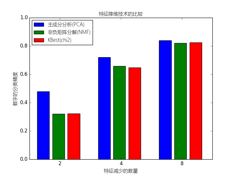
本例构建一个管道来进行降维和预测的工作:先降维,接着通过支持向量分类器进行预测.本例将演示与在网格搜索过程进行单变量特征选择相比,怎样使用GrideSearchCV和管道来优化单一的CV跑无监督的PCA降维与NMF降维不同类别评估器。

(原文:This example constructs a pipeline that does dimensionality reduction followed by prediction with a support vector classifier. It demonstrates the use of GridSearchCV and Pipeline to optimize over different classes of estimators in a single CV run – unsupervised PCA and NMF dimensionality reductions are compared to univariate feature selection during the grid search.)

# coding:utf-8

from __future__ import print_function, division
import numpy as np
from sklearn.datasets import load_digits
from sklearn.model_selection import GridSearchCV
from sklearn.pipeline import Pipeline
from sklearn.svm import LinearSVC
from sklearn.decomposition import PCA, NMF
from sklearn.feature_selection import SelectKBest, chi2
from pylab import *

pipe = Pipeline([
('reduce_dim', PCA()),
('classify', LinearSVC())
])

N_FEATURES_OPTIONS = [2, 4, 8]
C_OPTIONS = [1, 10, 100, 1000]
param_grid = [
{
'reduce_dim': [PCA(iterated_power=7), NMF()],
'reduce_dim__n_components': N_FEATURES_OPTIONS,
'classify__C': C_OPTIONS
},
{
'reduce_dim': [SelectKBest(chi2)],
'reduce_dim__k': N_FEATURES_OPTIONS,
'classify__C': C_OPTIONS
},
]
reducer_labels = [u'主成分分析(PCA)', u'非负矩阵分解(NMF)', u'KBest(chi2)']

grid = GridSearchCV(pipe, cv=3, n_jobs=2, param_grid=param_grid)
digits = load_digits()
grid.fit(digits.data, digits.target)

mean_scores = np.array(grid.cv_results_['mean_test_score'])
# 得分按照param_grid的迭代顺序,在这里就是字母顺序
mean_scores = mean_scores.reshape(len(C_OPTIONS), -1, len(N_FEATURES_OPTIONS))
# 为最优C选择分数
mean_scores = mean_scores.max(axis=0)
bar_offsets = (np.arange(len(N_FEATURES_OPTIONS)) *
(len(reducer_labels) + 1) + .5)

myfont = matplotlib.font_manager.FontProperties(fname="Microsoft-Yahei-UI-Light.ttc")
mpl.rcParams['axes.unicode_minus'] = False

plt.figure()
COLORS = 'bgrcmyk'
for i, (label, reducer_scores) in enumerate(zip(reducer_labels, mean_scores)):
plt.bar(bar_offsets + i, reducer_scores, label=label, color=COLORS[i])

plt.title(u"特征降维技术的比较",fontproperties=myfont)
plt.xlabel(u'特征减少的数量',fontproperties=myfont)
plt.xticks(bar_offsets + len(reducer_labels) / 2, N_FEATURES_OPTIONS)
plt.ylabel(u'数字的分类精度',fontproperties=myfont)
plt.ylim((0, 1))
plt.legend(loc='upper left',prop=myfont)
plt.show()