深度学习BP算法 BackPropagation以及详细例子解析
2016-09-29 19:53
302 查看
反向传播算法是多层神经网络的训练中举足轻重的算法,本文着重讲解方向传播算法的原理和推导过程。因此对于一些基本的神经网络的知识,本文不做介绍。在理解反向传播算法前,先要理解神经网络中的前馈神经网络算法。

给定一个前馈神经网络,我们用下面的记号来描述这个网络:
L:表示神经网络的层数;
nl:表示第l层神经元的个数;
fl(∙):表示l层神经元的激活函数;
Wl∈Rnl×nl−1:表示l−1层到第l层的权重矩阵;
bl∈Rnl:表示l−1层到l层的偏置;
zl∈Rnl:表示第l层神经元的输入;
al∈Rnl:表示第l层神经元的输出;
前馈神经网络通过如下的公式进行信息传播:
zl=Wl⋅al−1+blal=fl(zl)
上述两个公式可以合并写成如下形式:
zl=Wl⋅fl(zl−1)+bl
这样通过一层一层的信息传递,可以得到网络的最后输出y为:
x=a0→z1→a1→z1→⋯→aL−1→zL→aL=y
在推导反向传播的理论之前,首先看一幅能够直观的反映反向传播过程的图,这个图取材于Principles of training multi-layer neural network using back propagation。
Backpropagation is a common method for training a neural network. There is no
shortage of papers online that attempt to explain how backpropagation works, but few that include an example with actual numbers. This post is my attempt to explain how it works with a concrete example that folks can compare their own calculations to in
order to ensure they understand backpropagation correctly.
If this kind of thing interests you, you should sign
up for my newsletter where I post about AI-related projects that I’m working on.
You can play around with a Python script that I wrote that implements the backpropagation algorithm in this
Github repo.
For an interactive visualization showing a neural network as it learns, check out my Neural
Network visualization.
If you find this tutorial useful and want to continue learning about neural networks and their applications, I highly recommend checking out Adrian Rosebrock’s excellent tutorial on Getting
Started with Deep Learning and Python.
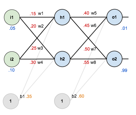
For this tutorial, we’re going to use a neural network with two inputs, two hidden neurons, two output neurons. Additionally, the hidden and output neurons will include a bias.
Here’s the basic structure:

In order to have some numbers to work with, here are the initial weights, the
biases, and training inputs/outputs:
The goal of backpropagation is to optimize the weights so that the neural network can learn how to correctly map arbitrary inputs to outputs.
For the rest of this tutorial we’re going to work with a single training set: given inputs 0.05 and 0.10, we want the neural network to output 0.01 and 0.99.
To begin, lets see what the neural network currently predicts given the weights and biases above and inputs of 0.05 and 0.10. To do this we’ll feed those inputs forward though the network.
We figure out the total net input to each hidden layer neuron, squash the
total net input using an activation function (here we use the logistic
function), then repeat the process with the output layer neurons.
Total net input is also referred to as just net input by some
sources.
Here’s how we calculate the total net input for

:


We then squash it using the logistic function to get the output of
:

Carrying out the same process for

we get:

We repeat this process for the output layer neurons, using the output from the hidden layer neurons as inputs.
Here’s the output for

:


And carrying out the same process for

we get:

We can now calculate the error for each output neuron using the squared
error function and sum them to get the total error:

Some
sources refer to the target as the ideal and the output as the actual.
The

is included
so that exponent is cancelled when we differentiate later on. The result is eventually multiplied by a learning rate anyway so it doesn’t matter that we introduce a constant here [1].
For example, the target output for
is 0.01 but
the neural network output 0.75136507, therefore its error is:

Repeating this process for
(remembering that the
target is 0.99) we get:

The total error for the neural network is the sum of these errors:

Our goal with backpropagation is to update each of the weights in the network so that they cause the actual output to be closer the target output, thereby minimizing the error for each output neuron and the network as a whole.
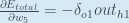
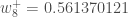
Consider

. We want to know how much a change in
affects
the total error, aka

.

is
read as “the partial derivative of

with
respect to

“. You can also say “the
gradient with respect to
“.
By applying the chain rule we
know that:

Visually, here’s what we’re doing:

We need to figure out each piece in this equation.
First, how much does the total error change with respect to the output?


is sometimes
expressed as

When we take the partial derivative of the total error with respect to

,
the quantity

becomes
zero because
does not affect
it which means we’re taking the derivative of a constant which is zero.
Next, how much does the output of
change with
respect to its total net input?
The partial derivative
of the logistic function is the output multiplied by 1 minus the output:


Finally, how much does the total net input of

change
with respect to
?

Putting it all together:


You’ll often see this calculation combined in the form of the delta
rule:

Alternatively, we have

and

which
can be written as

,
aka

(the Greek
letter delta) aka the node delta. We can use this to rewrite the calculation above:


Therefore:

Some sources extract the negative sign from

so
it would be written as:
To decrease the error, we then subtract this value from the current weight (optionally multiplied by some learning rate, eta, which we’ll set to 0.5):

Some sources use

(alpha)
to represent the learning rate, others
use

(eta), and others even
use

(epsilon).
We can repeat this process to get the new weights

,

,
and

:

We perform the actual updates in the neural network after we have the new weights leading into the hidden layer neurons (ie, we use the original weights, not the updated weights, when we continue the backpropagation algorithm below).
Next, we’ll continue the backwards pass by calculating new values for

,

,

,
and

.
Big picture, here’s what we need to figure out:

Visually:
We’re going to use a similar process as we did for the output layer, but slightly different to account for the fact that the output of each hidden layer neuron contributes to the output (and therefore error) of multiple output neurons. We know that

affects
both

and

therefore
the

needs
to take into consideration its effect on the both output neurons:

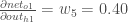
Starting with

:

We can calculate

using
values we calculated earlier:

And

is
equal to
:
Plugging them in:

Following the same process for

,
we get:

Therefore:

Now that we have
,
we need to figure out

and
then

for
each weight:

We calculate the partial derivative of the total net input to
with
respect to
the same as we did for the output
neuron:

Putting it all together:

You might also see this written as:


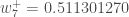
We can now update
:

Repeating this for
,
,
and
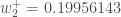

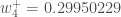
Finally, we’ve updated all of our weights! When we fed forward the 0.05 and 0.1 inputs originally, the error on the network was 0.298371109. After this first round of backpropagation, the total error is now down to 0.291027924. It might not seem like much,
but after repeating this process 10,000 times, for example, the error plummets to 0.000035085. At this point, when we feed forward 0.05 and 0.1, the two outputs neurons generate 0.015912196 (vs 0.01 target) and 0.984065734 (vs 0.99 target).
If you’ve made it this far and found any errors in any of the above or can think of any ways to make it clearer for future readers, don’t hesitate to drop
me a note. Thanks!
原文地址:http://blog.csdn.net/luxialan/article/details/42884227 https://mattmazur.com/2015/03/17/a-step-by-step-backpropagation-example/
前馈神经网络
如下图,是一个多层神经网络的简单示意图:给定一个前馈神经网络,我们用下面的记号来描述这个网络:
L:表示神经网络的层数;
nl:表示第l层神经元的个数;
fl(∙):表示l层神经元的激活函数;
Wl∈Rnl×nl−1:表示l−1层到第l层的权重矩阵;
bl∈Rnl:表示l−1层到l层的偏置;
zl∈Rnl:表示第l层神经元的输入;
al∈Rnl:表示第l层神经元的输出;
前馈神经网络通过如下的公式进行信息传播:
zl=Wl⋅al−1+blal=fl(zl)
上述两个公式可以合并写成如下形式:
zl=Wl⋅fl(zl−1)+bl
这样通过一层一层的信息传递,可以得到网络的最后输出y为:
x=a0→z1→a1→z1→⋯→aL−1→zL→aL=y
反向传播算法
在了解前馈神经网络的结构之后,我们一前馈神经网络的信息传递过程为基础,从而推到反向传播算法。首先要明确一点,反向传播算法是为了更好更快的训练前馈神经网络,得到神经网络每一层的权重参数和偏置参数。在推导反向传播的理论之前,首先看一幅能够直观的反映反向传播过程的图,这个图取材于Principles of training multi-layer neural network using back propagation。
Principles of training multi-layer neural network using backpropagation
| The project describes teaching process of multi-layer neural network employing backpropagation algorithm. To illustrate this process the three layer neural network with two inputs and one output,which is shown in the picture below, is used: 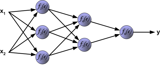 Each neuron is composed of two units. First unit adds products of weights coefficients and input signals. The second unit realise nonlinear function, called neuron activation function. Signal e is adder output signal, and y = f(e) is output signal of nonlinear element. Signal y is also output signal of neuron. 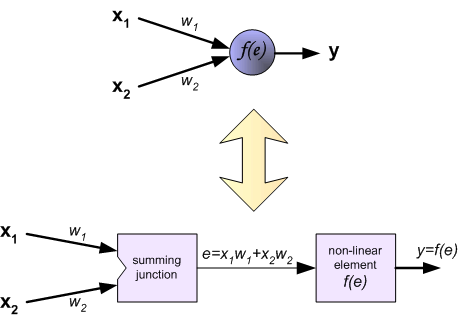 To teach the neural network we need training data set. The training data set consists of input signals (x1 and x2 ) assigned with corresponding target (desired output) z. The network training is an iterative process. In each iteration weights coefficients of nodes are modified using new data from training data set. Modification is calculated using algorithm described below: Each teaching step starts with forcing both input signals from training set. After this stage we can determine output signals values for each neuron in each network layer. Pictures below illustrate how signal is propagating through the network, Symbols w(xm)n represent weights of connections between network input xm and neuron n in input layer. Symbols yn represents output signal of neuron n. 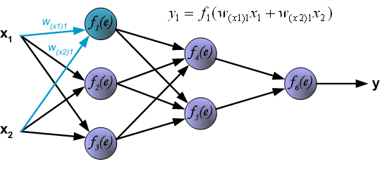 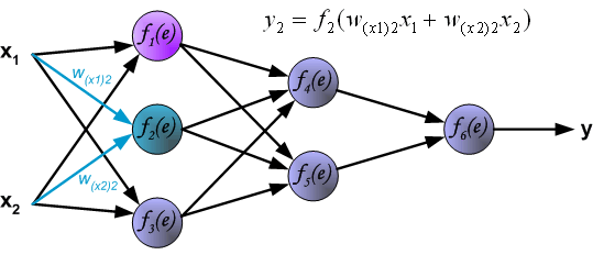 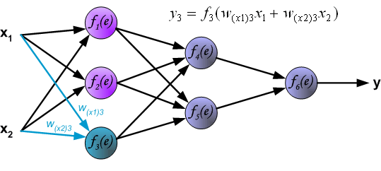 Propagation of signals through the hidden layer. Symbols wmn represent weights of connections between output of neuron m and input of neuron n in the next layer. 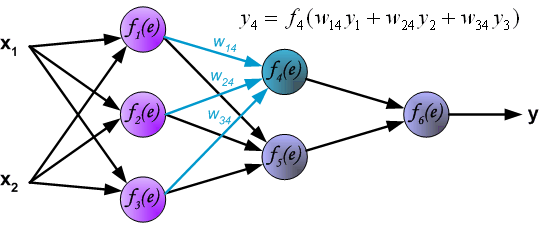 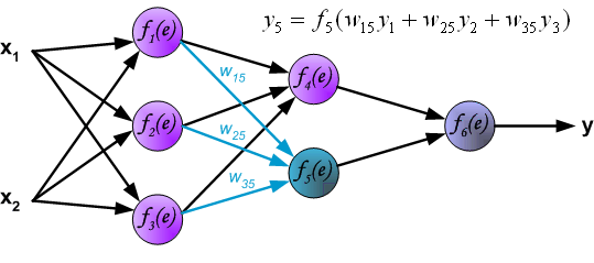 Propagation of signals through the output layer. 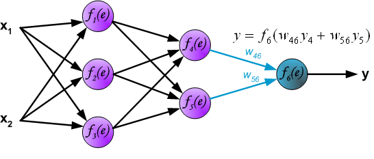 In the next algorithm step the output signal of the network y is compared with the desired output value (the target), which is found in training data set. The difference is called error signal d of output layer neuron. 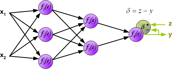 It is impossible to compute error signal for internal neurons directly, because output values of these neurons are unknown. For many years the effective method for training multiplayer networks has been unknown. Only in the middle eighties the backpropagation algorithm has been worked out. The idea is to propagate error signal d (computed in single teaching step) back to all neurons, which output signals were input for discussed neuron. 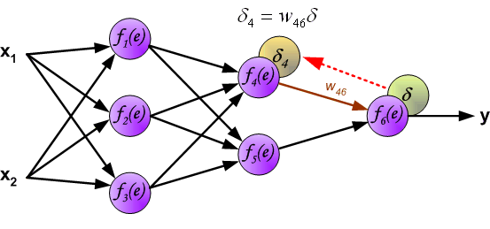 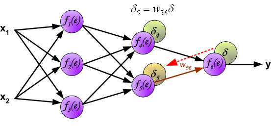 The weights' coefficients wmn used to propagate errors back are equal to this used during computing output value. Only the direction of data flow is changed (signals are propagated from output to inputs one after the other). This technique is used for all network layers. If propagated errors came from few neurons they are added. The illustration is below: 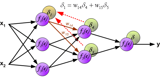 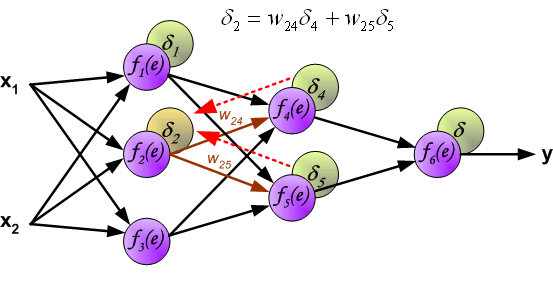 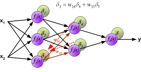 When the error signal for each neuron is computed, the weights coefficients of each neuron input node may be modified. In formulas below df(e)/de represents derivative of neuron activation function (which weights are modified). 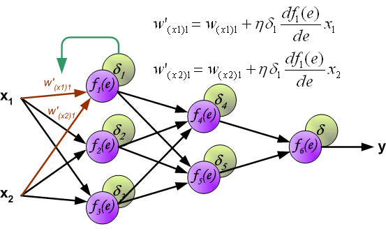 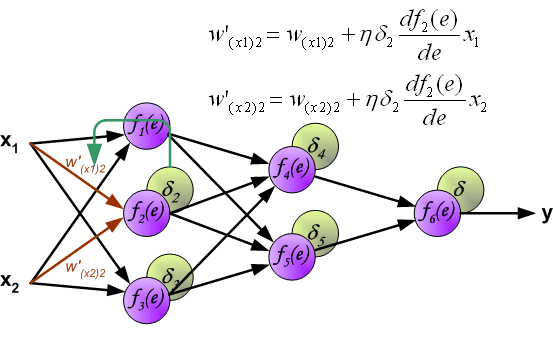 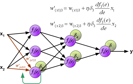 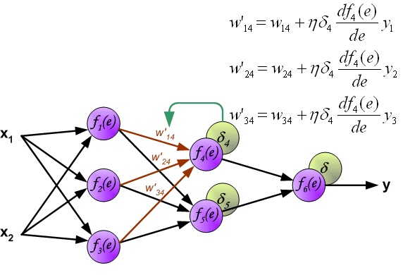 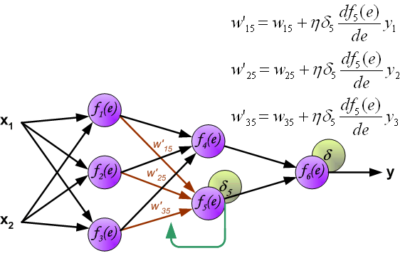 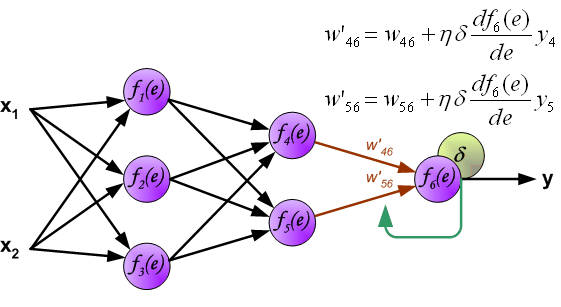 Coefficient h affects network teaching speed. There are a few techniques to select this parameter. The first method is to start teaching process with large value of the parameter. While weights coefficients are being established the parameter is being decreased gradually. The second, more complicated, method starts teaching with small parameter value. During the teaching process the parameter is being increased when the teaching is advanced and then decreased again in the final stage. Starting teaching process with low parameter value enables to determine weights coefficients signs. References Ryszard Tadeusiewcz "Sieci neuronowe", Kraków 1992 | ||
| Mariusz Bernacki Przemysław Włodarczyk mgr inż. Adam Gołda (2005) Katedra Elektroniki AGH | ||
| Last modified: 06.09.2004 Webmaster |
A Step by Step Backpropagation Example
Background
Backpropagation is a common method for training a neural network. There is noshortage of papers online that attempt to explain how backpropagation works, but few that include an example with actual numbers. This post is my attempt to explain how it works with a concrete example that folks can compare their own calculations to in
order to ensure they understand backpropagation correctly.
If this kind of thing interests you, you should sign
up for my newsletter where I post about AI-related projects that I’m working on.
Backpropagation in Python
You can play around with a Python script that I wrote that implements the backpropagation algorithm in thisGithub repo.
Backpropagation Visualization
For an interactive visualization showing a neural network as it learns, check out my NeuralNetwork visualization.
Additional Resources
If you find this tutorial useful and want to continue learning about neural networks and their applications, I highly recommend checking out Adrian Rosebrock’s excellent tutorial on GettingStarted with Deep Learning and Python.
Overview
For this tutorial, we’re going to use a neural network with two inputs, two hidden neurons, two output neurons. Additionally, the hidden and output neurons will include a bias.Here’s the basic structure:
In order to have some numbers to work with, here are the initial weights, the
biases, and training inputs/outputs:
The goal of backpropagation is to optimize the weights so that the neural network can learn how to correctly map arbitrary inputs to outputs.
For the rest of this tutorial we’re going to work with a single training set: given inputs 0.05 and 0.10, we want the neural network to output 0.01 and 0.99.
The Forward Pass
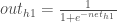
To begin, lets see what the neural network currently predicts given the weights and biases above and inputs of 0.05 and 0.10. To do this we’ll feed those inputs forward though the network.We figure out the total net input to each hidden layer neuron, squash the
total net input using an activation function (here we use the logistic
function), then repeat the process with the output layer neurons.
Total net input is also referred to as just net input by some
sources.
Here’s how we calculate the total net input for
:
We then squash it using the logistic function to get the output of
:
Carrying out the same process for
we get:
We repeat this process for the output layer neurons, using the output from the hidden layer neurons as inputs.
Here’s the output for
:
And carrying out the same process for
we get:
Calculating the Total Error
We can now calculate the error for each output neuron using the squarederror function and sum them to get the total error:
Some
sources refer to the target as the ideal and the output as the actual.
The
is included
so that exponent is cancelled when we differentiate later on. The result is eventually multiplied by a learning rate anyway so it doesn’t matter that we introduce a constant here [1].
For example, the target output for
is 0.01 but
the neural network output 0.75136507, therefore its error is:
Repeating this process for
(remembering that the
target is 0.99) we get:
The total error for the neural network is the sum of these errors:
The Backwards Pass
Our goal with backpropagation is to update each of the weights in the network so that they cause the actual output to be closer the target output, thereby minimizing the error for each output neuron and the network as a whole.
Output Layer
Consider . We want to know how much a change in
affects
the total error, aka
.
is
read as “the partial derivative of
with
respect to
“. You can also say “the
gradient with respect to
“.
By applying the chain rule we
know that:
Visually, here’s what we’re doing:
We need to figure out each piece in this equation.
First, how much does the total error change with respect to the output?
is sometimes
expressed as
When we take the partial derivative of the total error with respect to
,
the quantity
becomes
zero because
does not affect
it which means we’re taking the derivative of a constant which is zero.
Next, how much does the output of
change with
respect to its total net input?
The partial derivative
of the logistic function is the output multiplied by 1 minus the output:
Finally, how much does the total net input of
change
with respect to
?
Putting it all together:
You’ll often see this calculation combined in the form of the delta
rule:
Alternatively, we have
and
which
can be written as
,
aka
(the Greek
letter delta) aka the node delta. We can use this to rewrite the calculation above:
Therefore:
Some sources extract the negative sign from
so
it would be written as:
To decrease the error, we then subtract this value from the current weight (optionally multiplied by some learning rate, eta, which we’ll set to 0.5):
Some sources use
(alpha)
to represent the learning rate, others
use
(eta), and others even
use
(epsilon).
We can repeat this process to get the new weights
,
,
and
:
We perform the actual updates in the neural network after we have the new weights leading into the hidden layer neurons (ie, we use the original weights, not the updated weights, when we continue the backpropagation algorithm below).
Hidden Layer
Next, we’ll continue the backwards pass by calculating new values for ,
,
,
and
.
Big picture, here’s what we need to figure out:
Visually:

We’re going to use a similar process as we did for the output layer, but slightly different to account for the fact that the output of each hidden layer neuron contributes to the output (and therefore error) of multiple output neurons. We know that
affects
both
and
therefore
the
needs
to take into consideration its effect on the both output neurons:
Starting with
:
We can calculate
using
values we calculated earlier:
And
is
equal to
:
Plugging them in:
Following the same process for
,
we get:
Therefore:
Now that we have
,
we need to figure out
and
then
for
each weight:
We calculate the partial derivative of the total net input to
with
respect to
the same as we did for the output
neuron:
Putting it all together:
You might also see this written as:
We can now update
:
Repeating this for
,
,
and
Finally, we’ve updated all of our weights! When we fed forward the 0.05 and 0.1 inputs originally, the error on the network was 0.298371109. After this first round of backpropagation, the total error is now down to 0.291027924. It might not seem like much,
but after repeating this process 10,000 times, for example, the error plummets to 0.000035085. At this point, when we feed forward 0.05 and 0.1, the two outputs neurons generate 0.015912196 (vs 0.01 target) and 0.984065734 (vs 0.99 target).
If you’ve made it this far and found any errors in any of the above or can think of any ways to make it clearer for future readers, don’t hesitate to drop
me a note. Thanks!
原文地址:http://blog.csdn.net/luxialan/article/details/42884227 https://mattmazur.com/2015/03/17/a-step-by-step-backpropagation-example/

相关文章推荐
- 【深度学习】笔记3_caffe自带的第一个例子,Mnist手写数字识别所使用的LeNet网络模型的详细解释
- 传智博客佟老师jqurey学习笔记,以及例子代码详细注释。
- Caffe深度学习入门——配置caffe-SSD详细步骤以及填坑笔记
- 深度学习BP算法 BackPropagation
- 深度学习 16. 反向传递算法最简单的理解与提高,BP算法,Backpropagation, 自己的心得。
- Servlet上传文件详细解析以及注意事项
- c++ map 详细学习 例子
- ROR学习:《Web敏捷开发之道》例子添加购物车时发生的错误记录和解析
- j2me学习笔记【13】——创建矩形框、圆角矩形以及填充颜色小例子
- SAX简介以及例子学习
- 基于dwr2.0的Push推送技术详细解析以及实例
- 学习《详细解析Java中抽象类和接口的区别》笔记
- 8583详细解析,还有例子
- 基于dwr2.0的Push推送技术详细解析以及实例
- Servlet上传文件详细解析以及注意事项
- Servlet上传文件详细解析以及注意事项
- 动态绑定以及例子解析
- Android 简单例子以及入门学习资料链接
- iphone 开发Categories 、Extensions 以及相关应用(详细解析)
- Linux中编写自动编译的makefile的方法,以及详细解析。