基于Word2Vec Doc2Vec 进行文本情感分类
2016-09-06 21:58
591 查看
这篇文章介绍了使用Word2Vec和Doc2Vec进行文本情感分类,等后面有时间了再翻译一下:
Sentiment analysis is a common application of Natural Language Processing (NLP) methodologies, particularly classification, whose goal is to extract the emotional content in text. In this way, sentiment analysis can be seen as a method to quantify qualitative
data with some sentiment score. While sentiment is largely subjective, sentiment quantification has enjoyed many useful implementations, such as businesses gaining understanding about consumer reactions to a product, or detecting hateful speech in online comments.
The simplest form of sentiment analysis is to use a dictionary of good and bad words. Each word in a sentence has a score, typically +1 for positive sentiment and -1 for negative. Then, we simply add up the scores of all the words in the sentence to get a final
sentiment total. Clearly, this has many limitations, the most important being that it neglects context and surrounding words. For example, in our simple model the phrase “not good” may be classified as 0 sentiment, given “not” has a score of -1 and “good”
a score of +1. A human would likely classify “not good” as negative, despite the presence of “good”.
Another common method is to treat a text as a “bag of words”. We treat each text as a 1 by
where
value is the number of times that word appears. For example, the phrase “bag of bag of words” might be encoded as [2, 2, 1]. This could then be fed into a machine learning algorithm for classification, such as logistic regression or SVM, to predict sentiment
on unseen data. Note that this requires data with known sentiment to train on in a supervised fashion. While this is an improvement over the previous method, it still ignores context, and the size of the data increases with the size of the vocabulary.
Recently, Google developed a method called Word2Vec that captures the context of words, while at the same time reducing the size of the data. Word2Vec
is actually two different methods: Continuous Bag of Words (CBOW) and Skip-gram. In the CBOW method, the goal is to predict a word given the surrounding words. Skip-gram is the converse: we want to predict a window of words given a single word (see Figure
1). Both methods use artificial neural networks as their classification algorithm. Initially, each word in the vocabulary is a random N-dimensional vector. During training, the algorithm learns the optimal vector for each word using the CBOW or Skip-gram method.
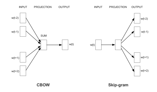
Figure 1: Architecture for the CBOW and Skip-gram method, taken from Efficient Estimation of Word Representations in Vector Space.
the current word, while
etc. are the surrounding words.
These word vectors now capture the context of surrounding words. This can be seen by using basic algebra to find word relations (i.e. “king” – “man” + “woman” = “queen”). These word vectors can be fed into a classification algorithm, as opposed to bag-of-words,
to predict sentiment. The advantage is that we now have some word context, and our feature space is much lower (typically ~300 as opposed to ~100,000, which is the size of our vocabulary). We also had to do very little manual feature creation since the neural
network was able to extract those features for us. Since text have varying length, one might take the average of all word vectors as the input to a classification algorithm to classify whole text documents.
However, even with the above method of averaging word vectors, we are ignoring word order. As a way to summarize bodies of text of varying length, Quoc Le and Tomas Mikolov came up with theDoc2Vec method.
This method is almost identical to Word2Vec, except we now generalize the method by adding a paragraph/document vector. Like Word2Vec, there are two methods: Distributed Memory (DM) and Distributed Bag of Words (DBOW). DM attempts to predict a word given its
previous words and a paragraph vector. Even though the context window moves across the text, the paragraph vector does not (hence distributed memory) and allows for some word-order to be captured. DBOW predicts a random group of words in a paragraph given
only its paragraph vector (see Figure 2).
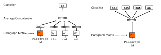
Figure 2: Architecture for Doc2Vec, taken from Distributed Representations of Sentences and Documents.
Once it has been trained, these paragraph vectors can be fed into a sentiment classifier without the need to aggregate words. This method is currently the state-of-the-art when it comes to sentiment classification on the IMDB movie review data set, achieving
only a 7.42% error rate. Of course, none of this is useful if we cannot actually implement them. Luckily, a very-well optimized version of Word2Vec and Doc2Vec is available in gensim,
a Python library.
In this section we show how one might use word vectors in a sentiment classification task. The
comes standard with the Anaconda distribution or can be installed using pip. From there you can train word vectors on your own corpus (a dataset of text documents) or import pre-trained vectors from C text or binary format:
I find this especially useful when loading Google’s pre-trained word vectors trained over ~100 billion words from the Google News dataset found in the "Pre-trained word and phrase vectors" section here.
Note that the file is ~3.5 GB unzipped. Using the Google word vectors we can see some interesting relationships between words:
What's interesting is that it can find grammatical relationships, for example identifying superlatives or verb stems:
"biggest" - "big" + "small" = "smallest"
"ate" - "eat" + "speak" = "spoke"
It's clear from the above examples that Word2Vec is able to learn non-trivial relationships between words. This is what makes them powerful for many NLP tasks, and in our case sentiment analysis. Before we move on to using them in sentiment analysis, let us
first examine Word2Vec's ability to separate and cluster words. We will use three example word sets: food, sports, and weather words taken from a wonderful website called Enchanted
Learning. Since these vectors are 300 dimensional, we will use Scikit-Learn's implementation of a dimensionality
reduction algorithm called t-SNE in order to visualize them in 2D.
First we have to obtain the word vectors as follows:
We can then use TSNE and matplotlib to visualize the clusters with the following code:
The result is as follows:
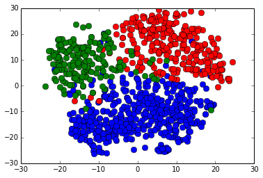
Figure 3: T-SNE projected clusters of food words (blue), sports words (red), and weather words (green).
We can see from the above that Word2Vec does a good job of separating unrelated words, as well as clustering together like words.
Now we will move on to an example in sentiment analysis with tweets gathered using emojis as search terms. We use these emojis as "fuzzy" labels for our data; a smiley emoji (
corresponds to positive sentiment, and a frowny (
data consists of an even split between positive and negative with a total of ~400,000 tweets. We randomly sample positive and negative tweets to construct an 80/20, train/test, split. We then train the Word2Vec model on the train tweets. In order to prevent
data leakage from the test set, we do not train Word2Vec on the test set until after our classifier has been fit on the training set. To construct inputs for our classifier, we take the average of all word vectors in a tweet. We will be using Scikit-Learn
to do a lot of the machine learning.
First we import our data and train the Word2Vec model.
Next we have to build word vectors for input text in order to average the value of all word vectors in the tweet using the following function:
Scaling moves our data set is part of the process of standardization where we move our dataset into a gaussian distribution with a mean of zero, meaning that values above the mean will be positive, and those below the mean will be negative. Many ML
models require scaled datasets to perform effectively, especially those with many features (like text classifiers).
Finally we have to build our test set vectors and scale them for evaluation.
Next we want to validate our classifier by calculating the prediction accuracy on test data, as well as examining its Receiver Operating Characteristic (ROC) curve. ROC curves measure the true-positive rate vs. the false-positive rate of a classifier while
adjusting a parameter of the model. In our case, we adjust the cut-off threshold probability for classifying a tweet as positive or negative sentiment. Generally, the larger the Area Under the Curve (AUC), the better our model does at maximizing true positives
while minimizing false positives. More on ROC curves can be found here.
To start we'll train our classifier, in this case using Stochastic Gradient Descent for Logistic Regression.
We'll then create the ROC curve for evaluation using matplotlib and the roc_curve method of Scikit-Learn's
The resulting curve is as follows:
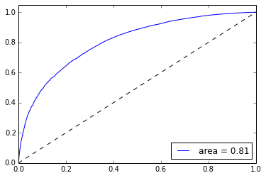
Figure 4: ROC Curve for a logistic classifier on our training data of tweets.
Without any type of feature creation and minimal text preprocessing we can achieve 73% test accuracy using a simple linear model provided by Scikit-Learn. Interestingly, removing punctuation actually causes the accuracy to suffer, suggesting Word2Vec can find
interesting features when characters such as "?" and "!" are present. Treating these as individual words, training for longer, doing more preprocessing, and adjusting parameters in both Word2Vec and the classifier could all help in improving accuracy. I have
found that using Artificial Neural Networks (ANNs) can improve the accuracy by about 5% when using word vectors. Note that Scikit-Learn does not provide an implementation of ANN classifiers so I used a custom library I created:
The resulting accuracy is 77%. As with any machine learning task, picking the right model is usually more a matter of art than science. If you'd like to use my custom library you can find it on my github.
Be warned, it is likely very messy and not regularly maintained! If you would like to contribute please feel free to fork the repository. It could definitely use some TLC!
Using the averages of word vectors worked fine in the case of tweets. This is because tweets are typically only a few to tens of words in length, which allows us to preserve the relevant features even when averaging. Once we go to the paragraph scale, however,
we risk throwing away rich features when we ignore word order and context. In this case it is better to use Doc2Vec to create our input features. As an example we will use the IMDB
movie review dataset to test the usefulness of Doc2Vec in sentiment analysis. The data consists of 25,000 positive movie reviews, 25,000 negative, and 50,000 unlabeled reviews. We first train Doc2Vec over the unlabeled reviews. The methodology then identically
follows that of the Word2Vec example above, except now we will use both DM and DBOW vectors as inputs by concatenating them.
These create LabeledSentence type objects:
Next we instantiate our two Doc2Vec models, DM and DBOW. The gensim documentation suggests training over the data multiple times and either adjusting the learning rate or randomizing the order of input at each pass. We then collect the movie review vectors
learned by the models.
Now we are ready to train a classifier over our review vectors. We will again use sklearn's SGDClassifier.
This model gives us a test accuracy of 0.86. We can also build a ROC curve for this classifier as follows:
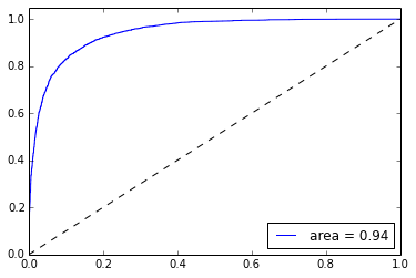
Figure 5: ROC Curve for a logistic classifier on our training data of IMDB movie reviews.
The original paper claimed they saw an improvement when using a 50 node neural network over a simple logistic regression classifier:
Interestingly, here we see no such improvement. The test accuracy is 0.85, and we do not approach their claimed test error of 7.42%. This could be for many reasons: we did not train for enough epochs over the training/test data, their implementation of Doc2Vec/ANN
is different, their hyperparameters are different, etc. It's hard to know exactly which since the paper does not go into great detail. In any case, we were able to obtain an 86% test accuracy with very little pre-processing and no feature creation/selection.
No fancy convolutions or treebanks necessary!
I hope you have seen not only the utility but ease of use for Word2Vec and Doc2Vec using standard tools like Python and gensim. With a very simple algorithm we can gain rich word and paragraph vectors that can be used in all kinds of NLP applications. What's
even better is Google's release of their own pre-trained word vectors trained on a much larger data set than anyone else can hope to obtain. If you want to train your own vectors over large data sets there is already an implementation of Word2Vec in Apache
Spark's MLlib. Happy NLP'ing!
A Word is Worth a Thousand Vectors
Word2Vec Tutorial
Gensim
Scikit-Learn: Working with Text Data
Natural Language Processing with Python
If you enjoyed this post and don't want to miss others like it, go to the blog home page and click theSubscribe button.
Michael Czerny
March 31, 2015
Subscribe
to this Blog
Share
Posted in: pythonnlp
Blog
Archive
District Data Labs
RSS
You can also find District Data Labs on Twitter, GitHub and Facebook.
© 2016 District Data Labs

转自:https://districtdatalabs.silvrback.com/modern-methods-for-sentiment-analysis
Sentiment analysis is a common application of Natural Language Processing (NLP) methodologies, particularly classification, whose goal is to extract the emotional content in text. In this way, sentiment analysis can be seen as a method to quantify qualitative
data with some sentiment score. While sentiment is largely subjective, sentiment quantification has enjoyed many useful implementations, such as businesses gaining understanding about consumer reactions to a product, or detecting hateful speech in online comments.
The simplest form of sentiment analysis is to use a dictionary of good and bad words. Each word in a sentence has a score, typically +1 for positive sentiment and -1 for negative. Then, we simply add up the scores of all the words in the sentence to get a final
sentiment total. Clearly, this has many limitations, the most important being that it neglects context and surrounding words. For example, in our simple model the phrase “not good” may be classified as 0 sentiment, given “not” has a score of -1 and “good”
a score of +1. A human would likely classify “not good” as negative, despite the presence of “good”.
Another common method is to treat a text as a “bag of words”. We treat each text as a 1 by
Nvector,
where
Nis the size of our vocabulary. Each column is a word, and the
value is the number of times that word appears. For example, the phrase “bag of bag of words” might be encoded as [2, 2, 1]. This could then be fed into a machine learning algorithm for classification, such as logistic regression or SVM, to predict sentiment
on unseen data. Note that this requires data with known sentiment to train on in a supervised fashion. While this is an improvement over the previous method, it still ignores context, and the size of the data increases with the size of the vocabulary.
Word2Vec and Doc2Vec
Recently, Google developed a method called Word2Vec that captures the context of words, while at the same time reducing the size of the data. Word2Vecis actually two different methods: Continuous Bag of Words (CBOW) and Skip-gram. In the CBOW method, the goal is to predict a word given the surrounding words. Skip-gram is the converse: we want to predict a window of words given a single word (see Figure
1). Both methods use artificial neural networks as their classification algorithm. Initially, each word in the vocabulary is a random N-dimensional vector. During training, the algorithm learns the optimal vector for each word using the CBOW or Skip-gram method.
Figure 1: Architecture for the CBOW and Skip-gram method, taken from Efficient Estimation of Word Representations in Vector Space.
W(t)is
the current word, while
w(t-2),
w(t-1),
etc. are the surrounding words.
These word vectors now capture the context of surrounding words. This can be seen by using basic algebra to find word relations (i.e. “king” – “man” + “woman” = “queen”). These word vectors can be fed into a classification algorithm, as opposed to bag-of-words,
to predict sentiment. The advantage is that we now have some word context, and our feature space is much lower (typically ~300 as opposed to ~100,000, which is the size of our vocabulary). We also had to do very little manual feature creation since the neural
network was able to extract those features for us. Since text have varying length, one might take the average of all word vectors as the input to a classification algorithm to classify whole text documents.
However, even with the above method of averaging word vectors, we are ignoring word order. As a way to summarize bodies of text of varying length, Quoc Le and Tomas Mikolov came up with theDoc2Vec method.
This method is almost identical to Word2Vec, except we now generalize the method by adding a paragraph/document vector. Like Word2Vec, there are two methods: Distributed Memory (DM) and Distributed Bag of Words (DBOW). DM attempts to predict a word given its
previous words and a paragraph vector. Even though the context window moves across the text, the paragraph vector does not (hence distributed memory) and allows for some word-order to be captured. DBOW predicts a random group of words in a paragraph given
only its paragraph vector (see Figure 2).
Figure 2: Architecture for Doc2Vec, taken from Distributed Representations of Sentences and Documents.
Once it has been trained, these paragraph vectors can be fed into a sentiment classifier without the need to aggregate words. This method is currently the state-of-the-art when it comes to sentiment classification on the IMDB movie review data set, achieving
only a 7.42% error rate. Of course, none of this is useful if we cannot actually implement them. Luckily, a very-well optimized version of Word2Vec and Doc2Vec is available in gensim,
a Python library.
Word2Vec Example in Python
In this section we show how one might use word vectors in a sentiment classification task. The gensimlibrary
comes standard with the Anaconda distribution or can be installed using pip. From there you can train word vectors on your own corpus (a dataset of text documents) or import pre-trained vectors from C text or binary format:
from gensim.models.word2vec import Word2Vec

model = Word2Vec.load_word2vec_format('vectors.txt', binary=False) #C text format
model = Word2Vec.load_word2vec_format('vectors.bin', binary=True) #C binary format
I find this especially useful when loading Google’s pre-trained word vectors trained over ~100 billion words from the Google News dataset found in the "Pre-trained word and phrase vectors" section here.
Note that the file is ~3.5 GB unzipped. Using the Google word vectors we can see some interesting relationships between words:
from gensim.models.word2vec import Word2Vec

model = Word2Vec.load_word2vec_format('GoogleNews-vectors-negative300.bin', binary=True)

model.most_similar(positive=['woman', 'king'], negative=['man'], topn=5)

[(u'queen', 0.711819589138031),
(u'monarch', 0.618967592716217),
(u'princess', 0.5902432799339294),
(u'crown_prince', 0.5499461889266968),
(u'prince', 0.5377323031425476)]
What's interesting is that it can find grammatical relationships, for example identifying superlatives or verb stems:
"biggest" - "big" + "small" = "smallest"
model.most_similar(positive=['biggest','small'], negative=['big'], topn=5)

[(u'smallest', 0.6086569428443909),
(u'largest', 0.6007465720176697),
(u'tiny', 0.5387299656867981),
(u'large', 0.456944078207016),
(u'minuscule', 0.43401968479156494)]
"ate" - "eat" + "speak" = "spoke"
model.most_similar(positive=['ate','speak'], negative=['eat'], topn=5)

[(u'spoke', 0.6965223550796509),
(u'speaking', 0.6261293292045593),
(u'conversed', 0.5754593014717102),
(u'spoken', 0.570488452911377),
(u'speaks', 0.5630602240562439)]
It's clear from the above examples that Word2Vec is able to learn non-trivial relationships between words. This is what makes them powerful for many NLP tasks, and in our case sentiment analysis. Before we move on to using them in sentiment analysis, let us
first examine Word2Vec's ability to separate and cluster words. We will use three example word sets: food, sports, and weather words taken from a wonderful website called Enchanted
Learning. Since these vectors are 300 dimensional, we will use Scikit-Learn's implementation of a dimensionality
reduction algorithm called t-SNE in order to visualize them in 2D.
First we have to obtain the word vectors as follows:
import numpy as np

with open('food_words.txt', 'r') as infile:
food_words = infile.readlines()

with open('sports_words.txt', 'r') as infile:
sports_words = infile.readlines()

with open('weather_words.txt', 'r') as infile:
weather_words = infile.readlines()

def getWordVecs(words):
vecs = []
for word in words:
word = word.replace('\n', '')
try:
vecs.append(model[word].reshape((1,300)))
except KeyError:
continue
vecs = np.concatenate(vecs)
return np.array(vecs, dtype='float') #TSNE expects float type values

food_vecs = getWordVecs(food_words)
sports_vecs = getWordVecs(sports_words)
weather_vecs = getWordVecs(weather_words)
We can then use TSNE and matplotlib to visualize the clusters with the following code:
from sklearn.manifold import TSNE
import matplotlib.pyplot as plt

ts = TSNE(2)
reduced_vecs = ts.fit_transform(np.concatenate((food_vecs, sports_vecs, weather_vecs)))

#color points by word group to see if Word2Vec can separate them
for i in range(len(reduced_vecs)):
if i < len(food_vecs):
#food words colored blue
color = 'b'
elif i >= len(food_vecs) and i < (len(food_vecs) + len(sports_vecs)):
#sports words colored red
color = 'r'
else:
#weather words colored green
color = 'g'
plt.plot(reduced_vecs[i,0], reduced_vecs[i,1], marker='o', color=color, markersize=8)
The result is as follows:
Figure 3: T-SNE projected clusters of food words (blue), sports words (red), and weather words (green).
We can see from the above that Word2Vec does a good job of separating unrelated words, as well as clustering together like words.
Analyzing the Sentiment of Emoji Tweets
Now we will move on to an example in sentiment analysis with tweets gathered using emojis as search terms. We use these emojis as "fuzzy" labels for our data; a smiley emoji (:-))
corresponds to positive sentiment, and a frowny (
:-() to negative. The
data consists of an even split between positive and negative with a total of ~400,000 tweets. We randomly sample positive and negative tweets to construct an 80/20, train/test, split. We then train the Word2Vec model on the train tweets. In order to prevent
data leakage from the test set, we do not train Word2Vec on the test set until after our classifier has been fit on the training set. To construct inputs for our classifier, we take the average of all word vectors in a tweet. We will be using Scikit-Learn
to do a lot of the machine learning.
First we import our data and train the Word2Vec model.
from sklearn.cross_validation import train_test_split
from gensim.models.word2vec import Word2Vec

with open('twitter_data/pos_tweets.txt', 'r') as infile:
pos_tweets = infile.readlines()

with open('twitter_data/neg_tweets.txt', 'r') as infile:
neg_tweets = infile.readlines()

#use 1 for positive sentiment, 0 for negative
y = np.concatenate((np.ones(len(pos_tweets)), np.zeros(len(neg_tweets))))

x_train, x_test, y_train, y_test = train_test_split(np.concatenate((pos_tweets, neg_tweets)), y, test_size=0.2)

#Do some very minor text preprocessing
def cleanText(corpus):
corpus = [z.lower().replace('\n','').split() for z in corpus]
return corpus

x_train = cleanText(x_train)
x_test = cleanText(x_test)

n_dim = 300
#Initialize model and build vocab
imdb_w2v = Word2Vec(size=n_dim, min_count=10)
imdb_w2v.build_vocab(x_train)

#Train the model over train_reviews (this may take several minutes)
imdb_w2v.train(x_train)
Next we have to build word vectors for input text in order to average the value of all word vectors in the tweet using the following function:
#Build word vector for training set by using the average value of all word vectors in the tweet, then scale
def buildWordVector(text, size):
vec = np.zeros(size).reshape((1, size))
count = 0.
for word in text:
try:
vec += imdb_w2v[word].reshape((1, size))
count += 1.
except KeyError:
continue
if count != 0:
vec /= count
return vec
Scaling moves our data set is part of the process of standardization where we move our dataset into a gaussian distribution with a mean of zero, meaning that values above the mean will be positive, and those below the mean will be negative. Many ML
models require scaled datasets to perform effectively, especially those with many features (like text classifiers).
from sklearn.preprocessing import scale
train_vecs = np.concatenate([buildWordVector(z, n_dim) for z in x_train])
train_vecs = scale(train_vecs)

#Train word2vec on test tweets
imdb_w2v.train(x_test)
Finally we have to build our test set vectors and scale them for evaluation.
#Build test tweet vectors then scale
test_vecs = np.concatenate([buildWordVector(z, n_dim) for z in x_test])
test_vecs = scale(test_vecs)
Next we want to validate our classifier by calculating the prediction accuracy on test data, as well as examining its Receiver Operating Characteristic (ROC) curve. ROC curves measure the true-positive rate vs. the false-positive rate of a classifier while
adjusting a parameter of the model. In our case, we adjust the cut-off threshold probability for classifying a tweet as positive or negative sentiment. Generally, the larger the Area Under the Curve (AUC), the better our model does at maximizing true positives
while minimizing false positives. More on ROC curves can be found here.
To start we'll train our classifier, in this case using Stochastic Gradient Descent for Logistic Regression.
#Use classification algorithm (i.e. Stochastic Logistic Regression) on training set, then assess model performance on test set
from sklearn.linear_model import SGDClassifier

lr = SGDClassifier(loss='log', penalty='l1')
lr.fit(train_vecs, y_train)

print 'Test Accuracy: %.2f'%lr.score(test_vecs, y_test)
We'll then create the ROC curve for evaluation using matplotlib and the roc_curve method of Scikit-Learn's
metricpackage.
#Create ROC curve
from sklearn.metrics import roc_curve, auc
import matplotlib.pyplot as plt

pred_probas = lr.predict_proba(test_vecs)[:,1]

fpr,tpr,_ = roc_curve(y_test, pred_probas)
roc_auc = auc(fpr,tpr)
plt.plot(fpr,tpr,label='area = %.2f' %roc_auc)
plt.plot([0, 1], [0, 1], 'k--')
plt.xlim([0.0, 1.0])
plt.ylim([0.0, 1.05])
plt.legend(loc='lower right')

plt.show()
The resulting curve is as follows:
Figure 4: ROC Curve for a logistic classifier on our training data of tweets.
Without any type of feature creation and minimal text preprocessing we can achieve 73% test accuracy using a simple linear model provided by Scikit-Learn. Interestingly, removing punctuation actually causes the accuracy to suffer, suggesting Word2Vec can find
interesting features when characters such as "?" and "!" are present. Treating these as individual words, training for longer, doing more preprocessing, and adjusting parameters in both Word2Vec and the classifier could all help in improving accuracy. I have
found that using Artificial Neural Networks (ANNs) can improve the accuracy by about 5% when using word vectors. Note that Scikit-Learn does not provide an implementation of ANN classifiers so I used a custom library I created:
from NNet import NeuralNet

nnet = NeuralNet(100, learn_rate=1e-1, penalty=1e-8)
maxiter = 1000
batch = 150
_ = nnet.fit(train_vecs, y_train, fine_tune=False, maxiter=maxiter, SGD=True, batch=batch, rho=0.9)

print 'Test Accuracy: %.2f'%nnet.score(test_vecs, y_test)
The resulting accuracy is 77%. As with any machine learning task, picking the right model is usually more a matter of art than science. If you'd like to use my custom library you can find it on my github.
Be warned, it is likely very messy and not regularly maintained! If you would like to contribute please feel free to fork the repository. It could definitely use some TLC!
Using Doc2Vec to Analyze Movie Reviews
Using the averages of word vectors worked fine in the case of tweets. This is because tweets are typically only a few to tens of words in length, which allows us to preserve the relevant features even when averaging. Once we go to the paragraph scale, however,we risk throwing away rich features when we ignore word order and context. In this case it is better to use Doc2Vec to create our input features. As an example we will use the IMDB
movie review dataset to test the usefulness of Doc2Vec in sentiment analysis. The data consists of 25,000 positive movie reviews, 25,000 negative, and 50,000 unlabeled reviews. We first train Doc2Vec over the unlabeled reviews. The methodology then identically
follows that of the Word2Vec example above, except now we will use both DM and DBOW vectors as inputs by concatenating them.
import gensim

LabeledSentence = gensim.models.doc2vec.LabeledSentence

from sklearn.cross_validation import train_test_split
import numpy as np

with open('IMDB_data/pos.txt','r') as infile:
pos_reviews = infile.readlines()

with open('IMDB_data/neg.txt','r') as infile:
neg_reviews = infile.readlines()

with open('IMDB_data/unsup.txt','r') as infile:
unsup_reviews = infile.readlines()

#use 1 for positive sentiment, 0 for negative
y = np.concatenate((np.ones(len(pos_reviews)), np.zeros(len(neg_reviews))))

x_train, x_test, y_train, y_test = train_test_split(np.concatenate((pos_reviews, neg_reviews)), y, test_size=0.2)

#Do some very minor text preprocessing
def cleanText(corpus):
punctuation = """.,?!:;(){}[]"""
corpus = [z.lower().replace('\n','') for z in corpus]
corpus = [z.replace('<br />', ' ') for z in corpus]

#treat punctuation as individual words
for c in punctuation:
corpus = [z.replace(c, ' %s '%c) for z in corpus]
corpus = [z.split() for z in corpus]
return corpus

x_train = cleanText(x_train)
x_test = cleanText(x_test)
unsup_reviews = cleanText(unsup_reviews)

#Gensim's Doc2Vec implementation requires each document/paragraph to have a label associated with it.
#We do this by using the LabeledSentence method. The format will be "TRAIN_i" or "TEST_i" where "i" is
#a dummy index of the review.
def labelizeReviews(reviews, label_type):
labelized = []
for i,v in enumerate(reviews):
label = '%s_%s'%(label_type,i)
labelized.append(LabeledSentence(v, [label]))
return labelized

x_train = labelizeReviews(x_train, 'TRAIN')
x_test = labelizeReviews(x_test, 'TEST')
unsup_reviews = labelizeReviews(unsup_reviews, 'UNSUP')
These create LabeledSentence type objects:
<gensim.models.doc2vec.LabeledSentence at 0xedd70b70>
Next we instantiate our two Doc2Vec models, DM and DBOW. The gensim documentation suggests training over the data multiple times and either adjusting the learning rate or randomizing the order of input at each pass. We then collect the movie review vectors
learned by the models.
import random

size = 400

#instantiate our DM and DBOW models
model_dm = gensim.models.Doc2Vec(min_count=1, window=10, size=size, sample=1e-3, negative=5, workers=3)
model_dbow = gensim.models.Doc2Vec(min_count=1, window=10, size=size, sample=1e-3, negative=5, dm=0, workers=3)

#build vocab over all reviews
model_dm.build_vocab(np.concatenate((x_train, x_test, unsup_reviews)))
model_dbow.build_vocab(np.concatenate((x_train, x_test, unsup_reviews)))

#We pass through the data set multiple times, shuffling the training reviews each time to improve accuracy.
all_train_reviews = np.concatenate((x_train, unsup_reviews))
for epoch in range(10):
perm = np.random.permutation(all_train_reviews.shape[0])
model_dm.train(all_train_reviews[perm])
model_dbow.train(all_train_reviews[perm])

#Get training set vectors from our models
def getVecs(model, corpus, size):
vecs = [np.array(model[z.labels[0]]).reshape((1, size)) for z in corpus]
return np.concatenate(vecs)

train_vecs_dm = getVecs(model_dm, x_train, size)
train_vecs_dbow = getVecs(model_dbow, x_train, size)

train_vecs = np.hstack((train_vecs_dm, train_vecs_dbow))

#train over test set
x_test = np.array(x_test)

for epoch in range(10):
perm = np.random.permutation(x_test.shape[0])
model_dm.train(x_test[perm])
model_dbow.train(x_test[perm])

#Construct vectors for test reviews
test_vecs_dm = getVecs(model_dm, x_test, size)
test_vecs_dbow = getVecs(model_dbow, x_test, size)

test_vecs = np.hstack((test_vecs_dm, test_vecs_dbow))
Now we are ready to train a classifier over our review vectors. We will again use sklearn's SGDClassifier.
from sklearn.linear_model import SGDClassifier

lr = SGDClassifier(loss='log', penalty='l1')
lr.fit(train_vecs, y_train)

print 'Test Accuracy: %.2f'%lr.score(test_vecs, y_test)
This model gives us a test accuracy of 0.86. We can also build a ROC curve for this classifier as follows:
#Create ROC curve
from sklearn.metrics import roc_curve, auc
%matplotlib inline
import matplotlib.pyplot as plt

pred_probas = lr.predict_proba(test_vecs)[:,1]

fpr,tpr,_ = roc_curve(y_test, pred_probas)
roc_auc = auc(fpr,tpr)
plt.plot(fpr,tpr,label='area = %.2f' %roc_auc)
plt.plot([0, 1], [0, 1], 'k--')
plt.xlim([0.0, 1.0])
plt.ylim([0.0, 1.05])
plt.legend(loc='lower right')

plt.show()
Figure 5: ROC Curve for a logistic classifier on our training data of IMDB movie reviews.
The original paper claimed they saw an improvement when using a 50 node neural network over a simple logistic regression classifier:
from NNet import NeuralNet

nnet = NeuralNet(50, learn_rate=1e-2)
maxiter = 500
batch = 150
_ = nnet.fit(train_vecs, y_train, fine_tune=False, maxiter=maxiter, SGD=True, batch=batch, rho=0.9)

print 'Test Accuracy: %.2f'%nnet.score(test_vecs, y_test)
Interestingly, here we see no such improvement. The test accuracy is 0.85, and we do not approach their claimed test error of 7.42%. This could be for many reasons: we did not train for enough epochs over the training/test data, their implementation of Doc2Vec/ANN
is different, their hyperparameters are different, etc. It's hard to know exactly which since the paper does not go into great detail. In any case, we were able to obtain an 86% test accuracy with very little pre-processing and no feature creation/selection.
No fancy convolutions or treebanks necessary!
Conclusion
I hope you have seen not only the utility but ease of use for Word2Vec and Doc2Vec using standard tools like Python and gensim. With a very simple algorithm we can gain rich word and paragraph vectors that can be used in all kinds of NLP applications. What'seven better is Google's release of their own pre-trained word vectors trained on a much larger data set than anyone else can hope to obtain. If you want to train your own vectors over large data sets there is already an implementation of Word2Vec in Apache
Spark's MLlib. Happy NLP'ing!
Additional Readings
A Word is Worth a Thousand VectorsWord2Vec Tutorial
Gensim
Scikit-Learn: Working with Text Data
Natural Language Processing with Python
If you enjoyed this post and don't want to miss others like it, go to the blog home page and click theSubscribe button.
Michael Czerny
March 31, 2015
Subscribe
to this Blog
Share
Posted in: pythonnlp
Read Next: Getting Started with Spark (in Python)
Blog Archive
District Data Labs
RSS
You can also find District Data Labs on Twitter, GitHub and Facebook.
© 2016 District Data Labs
转自:https://districtdatalabs.silvrback.com/modern-methods-for-sentiment-analysis

相关文章推荐
- spark 逻辑回归进行基于文本的分类预测
- 情感分析的新方法,使用word2vec对微博文本进行情感分析和分类
- 基于LSTM搭建一个文本情感分类的深度学习模型:准确率往往有95%以上
- python进行文本分类,基于word2vec,sklearn-svm对微博性别分类
- 基于SVM进行文本分类
- 分别使用sk-learn和mllib进行文本情感分类
- 【干货】--基于Python的文本情感分类
- 基于Attention Model的Aspect level文本情感分类---用Python+Keras实现
- 基于情感词典和朴素贝叶斯算法实现中文文本情感分类
- 基于情感词典的文本情感分类
- 基于朴素贝叶斯分类器的文本分类算法(上)
- LibSVM文本分类之工程中调用LibSVM进行文本分类
- 求做基于质心的半监督文本分类算法的同伴
- 借助weka实现的分类器进行针对文本分类问题的特征词选择实验(实验代码备份)
- 基于朴素贝叶斯分类器的文本分类算法(上)
- 基于朴素贝叶斯分类器的文本分类算法(上)
- 使用weka进行文本分类的例子
- 【转】基于朴素贝叶斯分类器的文本分类算法(下)
- 【转】 基于朴素贝叶斯分类器的文本分类算法(上)
- LibSVM文本分类之工程中调用LibSVM进行文本分类