#基于SVM的人脸识别

#数据说明

LFW全称为Labeled Faces in the Wild, 是一个应用于人脸识别问题的数据库，更多内容查看官方网站：http://vis-www.cs.umass.edu/lfw

LFW语料图片，每张图片都有人名Label标记。每个人可能有多张不同情况下情景下的图片。如George W Bush 有530张图片，而有一些人名对应的图片可能只有一张或者几张。我们将选取出现最多的人名作为人脸识别的类别，如本实验中选取出现频数超过70的人名为类别， 那么共计1288张图片。其中包括Ariel Sharon, Colin Powell, Donald Rumsfeld, George W Bush, Gerhard Schroeder, Hugo Chavez , Tony Blair等7个人名。

#问题描述

通过对7个人名的提取特征和标记，进行新输入的照片进行标记人名。这是一个多分类的问题，在本数据集合中类别数目为7. 这个问题的解决，不仅可以应用于像公司考勤一样少量人员的识别，也可以应用到新数据的标注中。语料库进一步标注，将进一步扩大训练数据集合数据量，从而进一步提高人脸识别的精确度。因此，对于图片的人名正确标注问题，或者这个多分类问题的研究和使用是有应用价值的。

#数据处理

训练与测试数据中样本数量为1288，对样本图片进行下采样后特征数为1850，所有人脸的Label数目为7。

首先将数据集划分为训练集合和测试集合，测试集合占25%(一般应该10%或者20%)，训练数据进行训练过程中，将分为训练集合和验证集合。通过验证集合选择最优模型，使用测试结合测试模型性能。

其次，通过对训练集合PCA分解，提取特征脸，提高训练速度，防止过度拟合。图片 1是关于不同的特征所占的总方差的比率关系，从中可以看出，关键特征主要集中在前50个。图片 2 是关于图片 1的累计分布图。从曲线中可以看出，当特征脸数目为50时，约占85%的数据信息，特征脸数据为100时，约占总信息量的90%左右。经过测试，最佳分类结果时，特征脸数目为80 .此时约占88%的总体方差。

print(__doc__)

import numpy as np
import matplotlib.pyplot as plt

from sklearn import linear_model, decomposition, datasets
from sklearn.pipeline import Pipeline
from sklearn.grid_search import GridSearchCV

logistic = linear_model.LogisticRegression()

pca = decomposition.PCA()
pipe = Pipeline(steps=[('pca', pca), ('logistic', logistic)])

digits = datasets.load_digits()
X_digits = digits.data
y_digits = digits.target

###############################################################################
# Plot the PCA spectrum
pca.fit(X_digits)

plt.figure(1, figsize=(4, 3))
plt.clf()
plt.axes([.2, .2, .7, .7])
plt.plot(pca.explained_variance_, linewidth=2)
plt.axis('tight')
plt.xlabel('n_components')
plt.ylabel('explained_variance_')

###############################################################################
# Prediction

n_components = [10, 20, 25, 30, 35, 40, 50, 64]#[i for i in range(1,65)]#
Cs = np.logspace(-4, 4, 3)

estimator = GridSearchCV(pipe,
dict(pca__n_components=n_components,
logistic__C=Cs))
estimator.fit(X_digits, y_digits)

plt.axvline(estimator.best_estimator_.named_steps['pca'].n_components,
linestyle=':', label='n_components chosen')
plt.legend(prop=dict(size=12))
plt.show()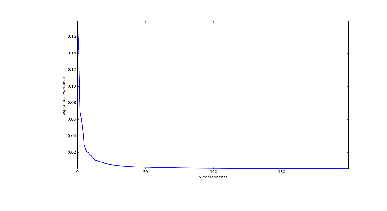

图片1: 不同特征选取数目的方差比率大小， 比率大小是按照从大到小的顺序排列的，从曲线中可以看出，最大的一维约占总体方差的18%



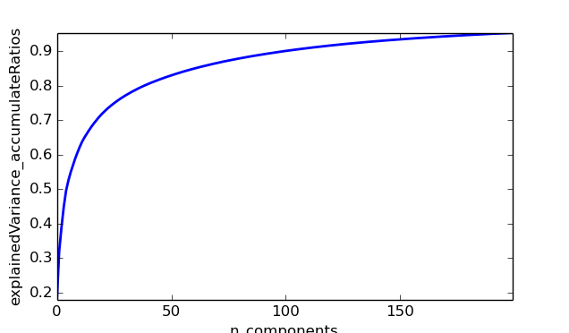
图片 2： 不同特征选取数目的方差累计比率曲线，从曲线中可以看出，当特征脸数目为50时，约占85%的数据信息，特征脸数据为100时，约占总信息量的90%左右经过测试，最佳分类结果时，特征脸数目为80.此时约占88%的总体方差。

因为不同的人有多个不同角度的照片，如果提取特征脸过多，会导致过度拟合，从而测试结果不理想，如果使用特征脸过少，则会导致人脸多类过程区分度不高而使得部分结果分类错误。而在LFW数据集合中，使用特征脸数目为80时效果最佳是可以理解的。图片 3 显示了前16个特征脸。



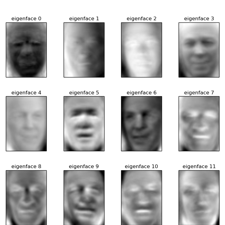
图片 3：对PCA降维度结果中16个特征脸先行呈现效果图

当然，数字图像处理常用的特征降维中NMF分解前几年取得了很多成果，有机会可以使用NMF分级进行特征提取和降维。

#模型训练与结果

训练代码

from __future__ import print_function

from time import time
import logging
import matplotlib.pyplot as plt

from sklearn.cross_validation import train_test_split
from sklearn.datasets import fetch_lfw_people
from sklearn.grid_search import GridSearchCV
from sklearn.metrics import classification_report
from sklearn.metrics import confusion_matrix
from sklearn.decomposition import RandomizedPCA
from sklearn.svm import SVC

print(__doc__)

# Display progress logs on stdout
logging.basicConfig(level=logging.INFO, format='%(asctime)s %(message)s')

###############################################################################
# Download the data, if not already on disk and load it as numpy arrays

lfw_people = fetch_lfw_people(min_faces_per_person=70, resize=0.4)

# introspect the images arrays to find the shapes (for plotting)
n_samples, h, w = lfw_people.images.shape

# for machine learning we use the 2 data directly (as relative pixel
# positions info is ignored by this model)
X = lfw_people.data
n_features = X.shape[1]

# the label to predict is the id of the person
y = lfw_people.target
target_names = lfw_people.target_names
n_classes = target_names.shape[0]

print("Total dataset size:")
print("n_samples: %d" % n_samples)
print("n_features: %d" % n_features)
print("n_classes: %d" % n_classes)

###############################################################################
# Split into a training set and a test set using a stratified k fold

# split into a training and testing set
X_train, X_test, y_train, y_test = train_test_split(
X, y, test_size=0.25, random_state=42)

###############################################################################
# Compute a PCA (eigenfaces) on the face dataset (treated as unlabeled
# dataset): unsupervised feature extraction / dimensionality reduction
n_components = 80

print("Extracting the top %d eigenfaces from %d faces"
% (n_components, X_train.shape[0]))
t0 = time()
pca = RandomizedPCA(n_components=n_components, whiten=True).fit(X_train)
print("done in %0.3fs" % (time() - t0))

eigenfaces = pca.components_.reshape((n_components, h, w))

print("Projecting the input data on the eigenfaces orthonormal basis")
t0 = time()
X_train_pca = pca.transform(X_train)
X_test_pca = pca.transform(X_test)
print("done in %0.3fs" % (time() - t0))

###############################################################################
# Train a SVM classification model

print("Fitting the classifier to the training set")
t0 = time()
param_grid = {'C': [1,10, 100, 500, 1e3, 5e3, 1e4, 5e4, 1e5],
'gamma': [0.0001, 0.0005, 0.001, 0.005, 0.01, 0.1], }
clf = GridSearchCV(SVC(kernel='rbf', class_weight='balanced'), param_grid)
clf = clf.fit(X_train_pca, y_train)
print("done in %0.3fs" % (time() - t0))
print("Best estimator found by grid search:")
print(clf.best_estimator_)

print(clf.best_estimator_.n_support_)
###############################################################################
# Quantitative evaluation of the model quality on the test set

print("Predicting people's names on the test set")
t0 = time()
y_pred = clf.predict(X_test_pca)
print("done in %0.3fs" % (time() - t0))

print(classification_report(y_test, y_pred, target_names=target_names))
print(confusion_matrix(y_test, y_pred, labels=range(n_classes)))

###############################################################################
# Qualitative evaluation of the predictions using matplotlib

def plot_gallery(images, titles, h, w, n_row=3, n_col=4):
"""Helper function to plot a gallery of portraits"""
plt.figure(figsize=(1.8 * n_col, 2.4 * n_row))
plt.subplots_adjust(bottom=0, left=.01, right=.99, top=.90, hspace=.35)
for i in range(n_row * n_col):
plt.subplot(n_row, n_col, i + 1)
# Show the feature face
plt.imshow(images[i].reshape((h, w)), cmap=plt.cm.gray)
plt.title(titles[i], size=12)
plt.xticks(())
plt.yticks(())

# plot the result of the prediction on a portion of the test set

def title(y_pred, y_test, target_names, i):
pred_name = target_names[y_pred[i]].rsplit(' ', 1)[-1]
true_name = target_names[y_test[i]].rsplit(' ', 1)[-1]
return 'predicted: %s\ntrue:      %s' % (pred_name, true_name)

prediction_titles = [title(y_pred, y_test, target_names, i)
for i in range(y_pred.shape[0])]

plot_gallery(X_test, prediction_titles, h, w)

# plot the gallery of the most significative eigenfaces

eigenface_titles = ["eigenface %d" % i for i in range(eigenfaces.shape[0])]
plot_gallery(eigenfaces, eigenface_titles, h, w)

plt.show()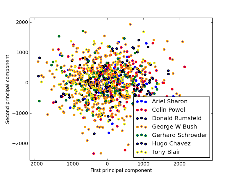

图片 4 实验数据在二维空间中分布情况，可以看出该数据集如果使用线性模型进行分类，效果将很差；我们将从非线性模型带核的SVM入手，解决该分类问题

分类模型将采用SVM分类器进行分类，其中核函数：

f=exp(−γ||x−x′||2)

我们将对核函数中的 γ 进行参数评估优化，此外对不同特征的权重进行优化，通过交叉验证和网格搜索方式，查找到最佳模型为γ=0.01， C = 10时，平均正确率达到90%，如表格 1所示。

表格 1: 关于测试集合人名标记结果的正确率，召回率和F1

#	Precision	Recall	F1	Support
Ariel Sharon	1.00	0.85	0.92	13
Colin Powell	0.86	0.95	0.90	60
Donald Rumsfeld	0.88	0.81	0.85	27
George W Bush	0.91	0.98	0.94	146
Gerhard Schroeder	0.95	0.72	0.82	25
Hugo Chavez	1.00	0.60	0.75	15
Tony Blair	0.91	0.86	0.89	36
Avg/Total	0.91	0.90	0.90	322

这么高的准确率，是由于我们仅仅选取了每个标识人名数目> 70的人名，但是大量的仅仅出现1次的人名存在。如果考虑这种数据稀疏性，将大大降低结果的准确率。但是，真实应用中，数据稀疏性问题是不得不考虑的问题。



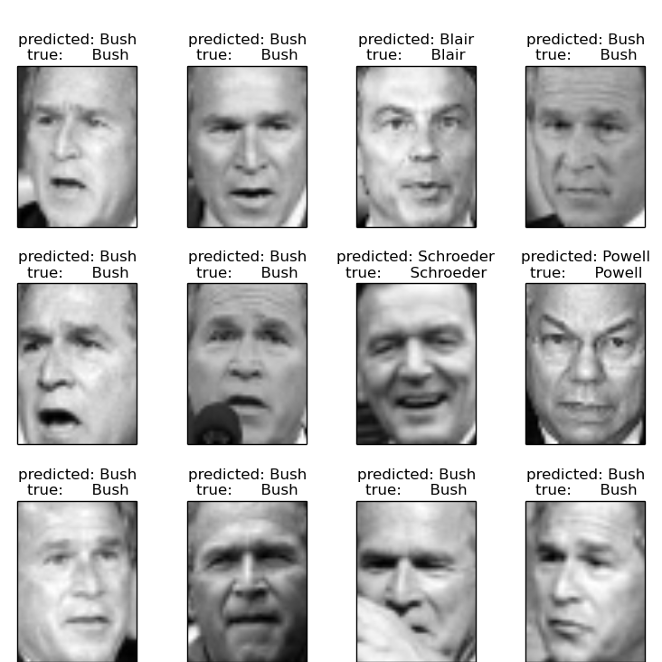
图片 5： 预测人名正确结果展示

#未来工作

本文中使用PCA实现特征脸提取，也可以使用其他特征提取方式进行降维。比如NMF实现矩阵分解在数字图像处理中的应用，实现NMF在人脸识别中的特征分解。当前使用的训练数据集使用的最小标记数据为70，当标记训练数据比较稀疏的时候，能否利用未标记数据提供正确率。后面的研究中将注意这两个方面的问题。

#参考文章

sklearnPCA

The Elements of Statistical Learning

Data Mining, Inference, and Prediction