学习大数据第四天：最小二乘法的Python实现

1.import numpy as np

np.pi

3.141592653589793

2. np.poly1d

numpy.poly1d

class numpy.poly1d(c_or_r, r=0, variable=None)[source]
A one-dimensional polynomial class.
A convenience class, used to encapsulate “natural” operations on polynomials so that said operations may take on their customary form in code (see Examples).

Parameters:

c_or_r : array_like The polynomial’s coefficients, in decreasing powers, or if the value of the second parameter is True, the polynomial’s roots (values where the polynomial evaluates to 0). For example, poly1d([1, 2, 3])returns an object that represents , whereas poly1d([1, 2, 3], True) returns one that represents . r : bool, optional If True, c_or_r specifies the polynomial’s roots; the default is False. variable : str, optional Changes the variable used when printing p from x to variable (see Examples).

Examples
Construct the polynomial

:

>>>

>>> p = np.poly1d([1, 2, 3])
>>> print np.poly1d(p)
2
1 x + 2 x + 3

Evaluate the polynomial at

:

>>>

>>> p(0.5)
4.25

Find the roots:

>>>

>>> p.r
array([-1.+1.41421356j, -1.-1.41421356j])
>>> p(p.r)
array([ -4.44089210e-16+0.j,  -4.44089210e-16+0.j])

These numbers in the previous line represent (0, 0) to machine precision
Show the coefficients:

>>>

>>> p.c
array([1, 2, 3])

Display the order (the leading zero-coefficients are removed):

>>>

>>> p.order
2

Show the coefficient of the k-th power in the polynomial (which is equivalent to p.c[-(i+1)]):

>>>

>>> p[1]
2

Polynomials can be added, subtracted, multiplied, and divided (returns quotient and remainder):

>>>

>>> p * p
poly1d([ 1,  4, 10, 12,  9])

>>>

>>> (p**3 + 4) / p
(poly1d([  1.,   4.,  10.,  12.,   9.]), poly1d([ 4.]))

asarray(p) gives
the coefficient array, so polynomials can be used in all functions that accept arrays:

>>>

>>> p**2 # square of polynomial
poly1d([ 1,  4, 10, 12,  9])

>>>

>>> np.square(p) # square of individual coefficients
array([1, 4, 9])

The variable used in the string representation of p can be modified, using the variable parameter:

>>>

>>> p = np.poly1d([1,2,3], variable='z')
>>> print p
2
1 z + 2 z + 3

Construct a polynomial from its roots:

>>>

>>> np.poly1d([1, 2], True)
poly1d([ 1, -3,  2])

This is the same polynomial as obtained by:

>>>

>>> np.poly1d([1, -1]) * np.poly1d([1, -2])
poly1d([ 1, -3,  2])

3.np.linspace

numpy.linspace

numpy.linspace(start, stop, num=50, endpoint=True, retstep=False, dtype=None)[source]
Return evenly spaced numbers over a specified interval.
Returns num evenly spaced samples, calculated over the interval [start, stop].
The endpoint of the interval can optionally be excluded.

Parameters:

start : scalar The starting value of the sequence. stop : scalar The end value of the sequence, unless endpoint is set to False. In that case, the sequence consists of all but the last of num + 1 evenly spaced samples, so that stop is excluded. Note that the step size changes when endpoint is False. num : int, optional Number of samples to generate. Default is 50. Must be non-negative. endpoint : bool, optional If True, stop is the last sample. Otherwise, it is not included. Default is True. retstep : bool, optional If True, return (samples, step), where step is the spacing between samples. dtype : dtype, optional The type of the output array. If dtype is not given, infer the data type from the other input arguments. New in version 1.9.0.

Returns:

samples : ndarray There are num equally spaced samples in the closed interval [start, stop] or the half-open interval[start, stop) (depending on whether endpoint is True or False). step : float Only returned if retstep is True Size of spacing between samples.

See also

arangeSimilar to linspace,
but uses a step size (instead of the number of samples).
logspaceSamples uniformly distributed in log space.

Examples

>>>

>>> np.linspace(2.0, 3.0, num=5)
array([ 2.  ,  2.25,  2.5 ,  2.75,  3.  ])
>>> np.linspace(2.0, 3.0, num=5, endpoint=False)
array([ 2. ,  2.2,  2.4,  2.6,  2.8])
>>> np.linspace(2.0, 3.0, num=5, retstep=True)
(array([ 2.  ,  2.25,  2.5 ,  2.75,  3.  ]), 0.25)

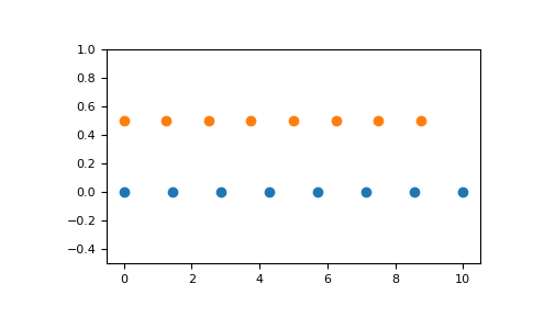
Graphical illustration:

>>>

>>> import matplotlib.pyplot as plt
>>> N = 8
>>> y = np.zeros(N)
>>> x1 = np.linspace(0, 10, N, endpoint=True)
>>> x2 = np.linspace(0, 10, N, endpoint=False)
>>> plt.plot(x1, y, 'o')
[<matplotlib.lines.Line2D object at 0x...>]
>>> plt.plot(x2, y + 0.5, 'o')
[<matplotlib.lines.Line2D object at 0x...>]
>>> plt.ylim([-0.5, 1])
(-0.5, 1)
>>> plt.show()

(Source code, png, pdf)