An Introduction to Machine Learning with Python
2016-04-15 00:25
946 查看
For the mind does not require filling like a bottle, but rather, like wood, it only requires kindling to create in it an impulse to think independently and an ardent desire for the
truth.
— Plutarch On Listening to
Lectures
The impulse to ingest more data is our first and most powerful instinct. Born with billions of neurons, as babies we begin developing complex synaptic networks by taking in massive amounts of data
- sounds, smells, tastes, textures, pictures. It's not always graceful, but it is an effective way to learn.
As data scientists, the trick is to encode similar learning instincts into applications, banking more on the volume of data that will flow through the system than on the elegance of the solution
(see also these discussions of the Netflix prize and the
"unreasonable effectiveness of data"). Building data products — or products that use data and generate more
data in return — requires the special ingredients of encoded learning and the ability to independently predict outcomes of new situations.
Fortunately Python and high level libraries like Scikit-learn, NLTK, PyBrain, Theano, and MLPy have made machine learning a lot more accessible than it would be otherwise. For better or worse, you
don't have to have an academic background in predictive methods to dip your toe into the machine learning waters (that said, we do encourage you to ML responsibly and have provided a list of helpful links and suggested further readings at the end). This post
aims to provide a basic introduction to machine learning: what it is, how it works, and how to get started with machine learning in Python using the Scikit-learn API.
Machine learning is, as artificial intelligence pioneer Arthur Samuel said,
a way of programming that gives computers "the ability to learn without being explicitly programmed.” In particular, it is a way to program computers to extract meaningful patterns from examples, and to use those patterns to make decisions or predictions.
In practice, this amounts to, first, creating a model with tunable parameters that can adjust themselves to the available data, then introducing new data and letting the model extrapolate. We also help the model balance between precisely capturing the behavior
of known data and generalizing enough to predict the behavior of unknown data.
In general, a learning problem considers a set of n known samples (we tend to call them instances). Instances are vector representations
of things in the real world. In a multidimensional decision space, we call each property of the vector representation an attribute or feature.
Machine learning essentially falls into three categories: supervised, unsupervised, and reinforcementlearning. The appropriate category
is determined by the type of data at hand, and depends largely on whether it is labeled or unlabeled.
Labeled data has, in addition to other features, a parameter of interest that can serve as the 'correct' answer. Unlabeled data does not have answers. With labeled data, we use supervised learning
methods. If the data does not have labels, we use unsupervised methods. For example, here is a well-known machine learning dataset, the Haberman
survival data, a record of cases from a study of the survival of breast cancer surgery patients between 1958 and 1970 at the University of Chicago's Billings Hospital.

Reinforcement learning methods such as swarms and genetic algorithms — where models interact with the environment for some reward — comprise a fascinating third category of machine learning, albeit
one beyond the scope of this post.
Below we'll explore several common techniques for supervised and unsupervised learning.
We can break supervised learning down further into two subcategories, regression problems andclassification problems. As with supervised
and unsupervised learning, the decision to use regression or classification is largely dictated by the type of data you have. If the labels in your dataset are continuous (e.g. percentages that indicate the probability of rain or fraud), your machine learning
problem likely calls for a regression technique. If the labels are discrete and the predictions should fall into categories (e.g. "male" or "female", "red", "green" or "blue"), it's a classification problem.
In the Haberman dataset shown above there are labels in addition to the three numerical features (the age of the patient at the time of her operation, the two-digit year of the patient's operation,
and the number of positive axillary nodes detected). The labels are categorical - a '1' indicates that the patient survived for more than five years after undergoing surgery to treat their cancer; a '2' indicates that the patient died within five years of
their surgery. So, if the goal is to predict a patient's five-year post-operative survival based on age, surgery year, and number of nodes, the best approach would be to build a classifier. However, if the labels were continuous (e.g. giving the number of
months of survival post operation), the problem might be better suited to regression.
Unsupervised learning is a way of discovering hidden structure in unlabeled data. Recall that with supervised learning, labels are the 'correct answers' that enable the model to adjust its parameters.
Unsupervised learning models have no such signal. Instead, unsupervised learning attempts to organize datasets into groups of similar data points, ensuring the groups are meaningfully dissimilar from each other. While an unsupervised learning algorithm is
unlikely to render clusters via a simple, elegantly parameterized equation like a human might, they can be strikingly successful at detecting patterns within datasets for which no human would even think to look.
There are two main approaches to clustering, partitive (or centroidal) and hierarchical, both of which separate data
into groups whose members share maximum similarity as defined (typically) by a distance metric. In partitive clustering, clusters are represented by central vectors, distributions, or densities. There are numerous variations of partitive clustering algorithms,
but some of the most common techniques include k-means, k-medoids, OPTICS, and affinity propagation. Hierarchical clustering involves creating clusters that have a predetermined ordering from top to bottom, and can be either agglomerative (clusters
begin as single instances and iteratively aggregate by similarity until all belong to a single group) or divisive (the dataset is gradually partitioned, beginning with all instances and finishing with single instances).
Scikit-learn is one of the extensions of SciPy (Scientific Python) that provides a wide variety of modern machine learning algorithms for classification, regression, clustering, feature extraction,
and optimization. It sits atop C libraries, LAPACK, LibSVM, and Cython, and provides extremely fast analysis for small- to medium-sized data sets. It is open source, commercially usable and is probably the best generalized machine learning framework currently
available. Some of Scikit-learn's features include: cross-validation, transformers, pipelining, grid search, model evaluation, generalized linear models, support vector machines, Bayes, decision trees, ensembles, clustering and density algorithms, and best
of all, a standard Python API. For this reason, Scikit-learn is often one of the first tools in a data scientist's toolkit.
Next we'll explore some regression, classification, and clustering models, but first install
The Scikit-learn API is an object-oriented interface centered around the concept of an
broadly any object that can learn from data, be it a classification, regression or clustering algorithm, or a transformer that extracts useful features from raw data. Each estimator in Scikit-learn has a fit and a predict method.
The
sets the state of the estimator based on the training data. Usually, the data is comprised of a two-dimensional numpy array X of shape (nsamples, npredictors) that holds the feature matrix, and a one-dimensional numpy array y that
holds the labels. Most estimators allow the user to control the fitting behavior, setting parameters when the estimator is instantiated or modifying them later.
predictions: predicted regression values in the case of regression, or the corresponding class labels in the case of classification. Classifiers that can predict the probability of class membership have a method
returns a two-dimensional numpy array of shape (nsamples, nclasses) where the classes are lexicographically ordered.
A
a special type of estimator that transforms input data by selecting a subset of the available features or extracting new features based on the original ones. Transformers can be used to normalize or scale features, or to impute missing values.
Scikit-learn also comes with a few datasets that can demonstrate the properties of classification and regression algorithms, as well as how the data should fit. The datasets module also contains
functions for loading data from the mldata.org repository as well as for generating random data. Coupled with the API, which allows you to rapidly deploy any number of models, these small toy datasets are helpful for getting started with machine learning.

Regressions are a type of supervised learning algorithm where, given continuous input features, the object is to predict the continuous target values.
Get started by loading some practice datasets from the Scikit-learn repository, on glucose
and insulin levels of diabetes patients and median home values in Boston:
Because they have continuous labels, both of these datasets lend themselves to regression. As we explore each of the predictive models below, we should be asking ourselves which performs the best
for each of the two sample datasets. To help with our evaluation, let's import some handy built-in tools from Scikit-learn; mean squared error, which indicates a regression model’s error in terms of precision (variance) and accuracy (bias),
and coefficient of determination or R2 score (a ratio of explained variance to total variance), which illustrates how well the prediction fits the data:
Linear Regression
A simple linear regression attempts to draw a straight line that will best minimize the residual sum of squares between the observations and the predictions.
Now we evaluate the fit of the model:
Try the same linear model with the Boston housing prices data:
Regularization: Ridge Regression
Regularization methods penalize the complexity of a model to limit overfitting and help with generalization. For example, ridge regression, also known
as Tikhonov regularization, penalizes a least squares regression model by shrinking the value of the regression coefficients. Compared to a standard linear regression, the slope will tend to be more stable and the variance
smaller.
Try the same regularization method with the Boston housing prices data:
Random Forest
Random forest is an ensemble method that creates a number of decision trees using the CART algorithm, each on a different subset of the data. The general approach to creating
the ensemble is bootstrap aggregation of the decision trees (also known as 'bagging').
And for the Boston dataset:

Given labeled input data (with two or more possible labels), classification aims to fit a function that can predict the discrete class of new input.
For our exploration of a few of the classification methods available in Scikit-learn, let's pick a new dataset to work with. Once you've exhausted the toy datasets available through the Scikit-learn
API, the next place to explore is the machine learning repository maintained by the University of California, Irvine. For the following
few examples, we'll be using the Haberman survival dataset we explored at the beginning of the post.
A Word on Cross-Validation
In supervised machine learning, data are divided into training and test sets. But what if certain chunks of the data have more variance than others? It's important to get into the habit of using
cross validation (we like to use 12 folds) to ensure that your models perform just as well regardless of the particular way the data are divided up.
To do this in
we'll import
As we explore different classifiers, we'll again be asking which model performs the best with our dataset. To help us evaluate, let's import
This will give us the precision, accuracy and recall scores for each classifier. Precision is the number of correct positive results divided by the number of all
positive results. Recall is the number of correct positive results divided by the number of positive results that should have been returned. The F1 scoreis a measure of a test's accuracy. It considers
both the precision and the recall of the test to compute the score. The F1 score can be interpreted as a weighted average of the precision and recall, where an F1 score reaches its best value at 1 and worst at 0.
Logistic Regression
A logistic regression mathematically calculates the decision boundary between the possibilities. It looks for a straight line that represents a cutoff that most
accurately represents the training data.
SVMs
Support vector machines (SVMs) use points in transformed problem space that separate the classes into groups. For data that is not linearly separable, mapping to a higher dimensional
feature space by computing the kernels can render the decision space more straightforward (this is called the "kernel trick"). Support vector machine models are versatile because they can be parameterized with a variety of different kernel functions including
linear, polynomial, sigmoid, and radial basis.
Random Forest
We used a Random Forest regressor in the previous section on Regression, but this ensemble method can also be used in classification. In fact, many supervised
models in Scikit-learn have both a regressor and a classifier version.

Clustering algorithms attempt to find patterns in unlabeled data. They are usually grouped into two main categories: centroidal (to find the centers of clusters) and hierarchical
(to find clusters of clusters).
In order to explore clustering, let's pull another dataset from the UCI repository, this one on grocery
store customer spending behavior:
K-Means Clustering
K-Means Clustering partitions N samples into k clusters, where each sample belongs to a cluster to which it has the closest mean of its neighbors. This problem is "NP-hard",
but there are good estimations.
Now plot the results:
The black dots are our data points and the x's represent the centers of the clusters that were identified by our model:

Scikit-learn includes a lot of useful clustering models, which, as you
experiment, you'll find perform better and worse depending on the number of clusters, density of the data, dimensionality, and desired distance metric.
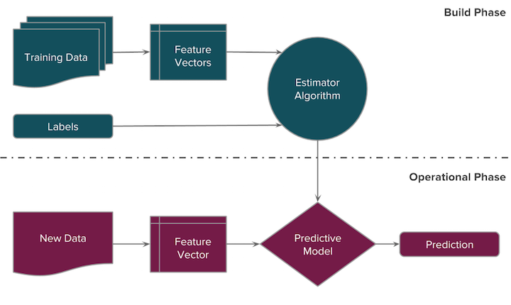
When we talk about data science and the data science pipeline, we are typically talking about the management of data flows for a specific purpose - the modeling of some hypothesis. Those models
we construct can then be used in data products as an engine to create useful new data, as shown in the below pipeline:
The general model workflow for conducting machine learning tasks is as follows. Keep in mind that the best results will often be obtained through numerous iterations of steps 2-6.
Acquire the data - Choose data that will help you solve a problem or seems otherwise interesting. Perform initial descriptive analysis.
Prepare your data - Resolve missing values, remove outliers, and transform text fields to numeric values. For supervised learning you will
have an input matrix, where each row is an observation and each column is a predictor, as well as output data in a numerical vector, character array, etc.
Choose your learning algorithm - Decide what you want in your algorithm (speed, interpretability, accuracy, good memory management, implementability).
Pick one algorithm or a collection; the Sckit-learn API easily allows you to use multiple models with the same input and compare the results.
Fit your model - See code snippets above!
Pick a validation method and examine the "fit", updating if necessary - Decide how you will measure error. If you want a better fit, try tuning
the model parameters, adjusting your regularization or bias variable, or picking a new algorithm all together.
Use your model for prediction on new data
The wide range of toy datsets in the UCI Machine Learning Repository make it pretty easy (almost too easy...) for those new to machine learning to get started. In order to fully operationalize Scikit-learn,
most datasets will require significant preprocessing, including the transformer estimators mentioned in the API discussion, as well as substantial data exploration, wrangling and
feature engineering. For instance, if you're trying to use machine learning methods with text data (perhaps to do sentiment
analysis), you'll have to convert the words to vectors.
Nevertheless, the Scikit-learn API makes machine learning very straightforward, and facilitates exploration with many different types of models. Depending on the dataset, some models will dramatically
outperform others. The best approach, particularly for those just getting started with machine learning in Python, is to check out Scikit-learn's handy flowchart,
experiment with grid search, and try out many different models (and the available parameters) until you begin to develop a bit of intuition
around model selection and tuning. Coupled with the further readings listed below, you should be dangerous in no time.
Wondering how to get your (non-toy) dataset into better shape for modeling? Looking for more on determining which model is best for your data? Stay tuned for upcoming posts exploring pipelining
with Scikit-learn and visual diagnostics for model evaluation!
Scikit-learn
UCI Machine Learning Repository
Neural networks online class
Kaggle challenges
Andrew Ng's course notes
Scikit-learn: Machine Learning in Python by F. Pedregrosa et al. (2011)
API design for machine learning software by L. Buitinck et al. (2013)
Thoughtful Machine Learning by M. Kirk (2011)
Pattern Recognition and Machine Learning by C. Bishop (2007)
Programming Collective Intelligence by T. Segaran (2007)
Learning Scikit-learn by R. Garreta and G. Moncecchi (2013)
Building Machine Learning Systems with Python by W. Richert (2013)
Applied Regression Analysis and Generalized Linear Models, 3rd ed. by J. Fox (2015)
As always, if you liked this post, please subscribe to the DDL blog by clicking the Subscribe button below and make sure to follow us on Facebook and Twitter.
And finally, a sincere thank you to Benjamin Bengfort and Gianna Capezio for their thoughtful editorial guidance and contributions to this post!
You might also be interested in these articles...
truth.
— Plutarch On Listening to
Lectures
The impulse to ingest more data is our first and most powerful instinct. Born with billions of neurons, as babies we begin developing complex synaptic networks by taking in massive amounts of data
- sounds, smells, tastes, textures, pictures. It's not always graceful, but it is an effective way to learn.
As data scientists, the trick is to encode similar learning instincts into applications, banking more on the volume of data that will flow through the system than on the elegance of the solution
(see also these discussions of the Netflix prize and the
"unreasonable effectiveness of data"). Building data products — or products that use data and generate more
data in return — requires the special ingredients of encoded learning and the ability to independently predict outcomes of new situations.
Fortunately Python and high level libraries like Scikit-learn, NLTK, PyBrain, Theano, and MLPy have made machine learning a lot more accessible than it would be otherwise. For better or worse, you
don't have to have an academic background in predictive methods to dip your toe into the machine learning waters (that said, we do encourage you to ML responsibly and have provided a list of helpful links and suggested further readings at the end). This post
aims to provide a basic introduction to machine learning: what it is, how it works, and how to get started with machine learning in Python using the Scikit-learn API.
What is Machine Learning?
Machine learning is, as artificial intelligence pioneer Arthur Samuel said,a way of programming that gives computers "the ability to learn without being explicitly programmed.” In particular, it is a way to program computers to extract meaningful patterns from examples, and to use those patterns to make decisions or predictions.
In practice, this amounts to, first, creating a model with tunable parameters that can adjust themselves to the available data, then introducing new data and letting the model extrapolate. We also help the model balance between precisely capturing the behavior
of known data and generalizing enough to predict the behavior of unknown data.
In general, a learning problem considers a set of n known samples (we tend to call them instances). Instances are vector representations
of things in the real world. In a multidimensional decision space, we call each property of the vector representation an attribute or feature.
Types of Machine Learning
Machine learning essentially falls into three categories: supervised, unsupervised, and reinforcementlearning. The appropriate categoryis determined by the type of data at hand, and depends largely on whether it is labeled or unlabeled.
Labeled data has, in addition to other features, a parameter of interest that can serve as the 'correct' answer. Unlabeled data does not have answers. With labeled data, we use supervised learning
methods. If the data does not have labels, we use unsupervised methods. For example, here is a well-known machine learning dataset, the Haberman
survival data, a record of cases from a study of the survival of breast cancer surgery patients between 1958 and 1970 at the University of Chicago's Billings Hospital.
Reinforcement learning methods such as swarms and genetic algorithms — where models interact with the environment for some reward — comprise a fascinating third category of machine learning, albeit
one beyond the scope of this post.
Below we'll explore several common techniques for supervised and unsupervised learning.
Supervised Learning: Regression and Classification
We can break supervised learning down further into two subcategories, regression problems andclassification problems. As with supervisedand unsupervised learning, the decision to use regression or classification is largely dictated by the type of data you have. If the labels in your dataset are continuous (e.g. percentages that indicate the probability of rain or fraud), your machine learning
problem likely calls for a regression technique. If the labels are discrete and the predictions should fall into categories (e.g. "male" or "female", "red", "green" or "blue"), it's a classification problem.
In the Haberman dataset shown above there are labels in addition to the three numerical features (the age of the patient at the time of her operation, the two-digit year of the patient's operation,
and the number of positive axillary nodes detected). The labels are categorical - a '1' indicates that the patient survived for more than five years after undergoing surgery to treat their cancer; a '2' indicates that the patient died within five years of
their surgery. So, if the goal is to predict a patient's five-year post-operative survival based on age, surgery year, and number of nodes, the best approach would be to build a classifier. However, if the labels were continuous (e.g. giving the number of
months of survival post operation), the problem might be better suited to regression.
Unsupervised Learning: Clustering
Unsupervised learning is a way of discovering hidden structure in unlabeled data. Recall that with supervised learning, labels are the 'correct answers' that enable the model to adjust its parameters.Unsupervised learning models have no such signal. Instead, unsupervised learning attempts to organize datasets into groups of similar data points, ensuring the groups are meaningfully dissimilar from each other. While an unsupervised learning algorithm is
unlikely to render clusters via a simple, elegantly parameterized equation like a human might, they can be strikingly successful at detecting patterns within datasets for which no human would even think to look.
There are two main approaches to clustering, partitive (or centroidal) and hierarchical, both of which separate data
into groups whose members share maximum similarity as defined (typically) by a distance metric. In partitive clustering, clusters are represented by central vectors, distributions, or densities. There are numerous variations of partitive clustering algorithms,
but some of the most common techniques include k-means, k-medoids, OPTICS, and affinity propagation. Hierarchical clustering involves creating clusters that have a predetermined ordering from top to bottom, and can be either agglomerative (clusters
begin as single instances and iteratively aggregate by similarity until all belong to a single group) or divisive (the dataset is gradually partitioned, beginning with all instances and finishing with single instances).
Scikit-learn
Scikit-learn is one of the extensions of SciPy (Scientific Python) that provides a wide variety of modern machine learning algorithms for classification, regression, clustering, feature extraction,and optimization. It sits atop C libraries, LAPACK, LibSVM, and Cython, and provides extremely fast analysis for small- to medium-sized data sets. It is open source, commercially usable and is probably the best generalized machine learning framework currently
available. Some of Scikit-learn's features include: cross-validation, transformers, pipelining, grid search, model evaluation, generalized linear models, support vector machines, Bayes, decision trees, ensembles, clustering and density algorithms, and best
of all, a standard Python API. For this reason, Scikit-learn is often one of the first tools in a data scientist's toolkit.
Next we'll explore some regression, classification, and clustering models, but first install
Scikit-learnusing
pip:
$ pip install scikit-learn
The Scikit-learn API
The Scikit-learn API is an object-oriented interface centered around the concept of an Estimator—
broadly any object that can learn from data, be it a classification, regression or clustering algorithm, or a transformer that extracts useful features from raw data. Each estimator in Scikit-learn has a fit and a predict method.
The
Estimator.fitmethod
sets the state of the estimator based on the training data. Usually, the data is comprised of a two-dimensional numpy array X of shape (nsamples, npredictors) that holds the feature matrix, and a one-dimensional numpy array y that
holds the labels. Most estimators allow the user to control the fitting behavior, setting parameters when the estimator is instantiated or modifying them later.
Estimator.predictgenerates
predictions: predicted regression values in the case of regression, or the corresponding class labels in the case of classification. Classifiers that can predict the probability of class membership have a method
Estimator.predict_probathat
returns a two-dimensional numpy array of shape (nsamples, nclasses) where the classes are lexicographically ordered.
A
transformeris
a special type of estimator that transforms input data by selecting a subset of the available features or extracting new features based on the original ones. Transformers can be used to normalize or scale features, or to impute missing values.
Scikit-learn also comes with a few datasets that can demonstrate the properties of classification and regression algorithms, as well as how the data should fit. The datasets module also contains
functions for loading data from the mldata.org repository as well as for generating random data. Coupled with the API, which allows you to rapidly deploy any number of models, these small toy datasets are helpful for getting started with machine learning.
Models in Scikit-learn
Regression
Regressions are a type of supervised learning algorithm where, given continuous input features, the object is to predict the continuous target values.
Get started by loading some practice datasets from the Scikit-learn repository, on glucose
and insulin levels of diabetes patients and median home values in Boston:
from sklearn.datasets import load_diabetes
from sklearn.datasets import load_boston

diabetes = load_diabetes()
boston = load_boston()
Because they have continuous labels, both of these datasets lend themselves to regression. As we explore each of the predictive models below, we should be asking ourselves which performs the best
for each of the two sample datasets. To help with our evaluation, let's import some handy built-in tools from Scikit-learn; mean squared error, which indicates a regression model’s error in terms of precision (variance) and accuracy (bias),
and coefficient of determination or R2 score (a ratio of explained variance to total variance), which illustrates how well the prediction fits the data:
from sklearn.metrics import mean_squared_error as mse
from sklearn.metrics import r2_score
Linear Regression
A simple linear regression attempts to draw a straight line that will best minimize the residual sum of squares between the observations and the predictions.
from sklearn.linear_model import LinearRegression

model = LinearRegression()
model.fit(diabetes.data, diabetes.target) # Remember, each Estimator in Scikit-learn has a fit method

expected = diabetes.target
predicted = model.predict(diabetes.data) # ...and also a predict method.
Now we evaluate the fit of the model:
print "Linear regression model \n Diabetes dataset"
print "Mean squared error = %0.3f" % mse(expected, predicted)
print "R2 score = %0.3f" % r2_score(expected, predicted)
Try the same linear model with the Boston housing prices data:
model.fit(boston.data, boston.target)

expected = boston.target
predicted = model.predict(boston.data)

print "Linear regression model \n Boston dataset"
print "Mean squared error = %0.3f" % mse(expected, predicted)
print "R2 score = %0.3f" % r2_score(expected, predicted)
Regularization: Ridge Regression
Regularization methods penalize the complexity of a model to limit overfitting and help with generalization. For example, ridge regression, also known
as Tikhonov regularization, penalizes a least squares regression model by shrinking the value of the regression coefficients. Compared to a standard linear regression, the slope will tend to be more stable and the variance
smaller.
from sklearn.linear_model import Ridge

model = Ridge(alpha=0.1)
model.fit(diabetes.data, diabetes.target)

expected = diabetes.target
predicted = model.predict(diabetes.data)

print "Ridge regression model \n Diabetes dataset"
print "Mean squared error = %0.3f" % mse(expected, predicted)
print "R2 score = %0.3f" % r2_score(expected, predicted)
Try the same regularization method with the Boston housing prices data:
model.fit(boston.data, boston.target)

expected = boston.target
predicted = model.predict(boston.data)

print "Ridge regression model \n Boston dataset"
print "Mean squared error = %0.3f" % mse(expected, predicted)
print "R2 score = %0.3f" % r2_score(expected, predicted)
Random Forest
Random forest is an ensemble method that creates a number of decision trees using the CART algorithm, each on a different subset of the data. The general approach to creating
the ensemble is bootstrap aggregation of the decision trees (also known as 'bagging').
from sklearn.ensemble import RandomForestRegressor

model = RandomForestRegressor()
model.fit(diabetes.data, diabetes.target)

expected = diabetes.target
predicted = model.predict(diabetes.data)

print "Random Forest model \n Diabetes dataset"
print "Mean squared error = %0.3f" % mse(expected, predicted)
print "R2 score = %0.3f" % r2_score(expected, predicted)
And for the Boston dataset:
model.fit(boston.data, boston.target)

expected = boston.target
predicted = model.predict(boston.data)

print "Random Forest model \n Boston dataset"
print "Mean squared error = %0.3f" % mse(expected, predicted)
print "R2 score = %0.3f" % r2_score(expected, predicted)
Classification
Given labeled input data (with two or more possible labels), classification aims to fit a function that can predict the discrete class of new input.
For our exploration of a few of the classification methods available in Scikit-learn, let's pick a new dataset to work with. Once you've exhausted the toy datasets available through the Scikit-learn
API, the next place to explore is the machine learning repository maintained by the University of California, Irvine. For the following
few examples, we'll be using the Haberman survival dataset we explored at the beginning of the post.
import os
import requests
import pandas as pd

URL = "https://archive.ics.uci.edu/ml/machine-learning-databases/haberman/haberman.data"
response = requests.get(URL)
outpath = os.path.abspath("haberman.txt")
with open(outpath, 'w') as f:
f.write(response.content)

df = pd.read_csv("haberman.txt", header=None, names=["age_at_op","op_yr","nr_nodes","survival"])
FEATURES = df[["age_at_op","op_yr","nr_nodes"]]
TARGETS = df[["survival"]]
A Word on Cross-Validation
In supervised machine learning, data are divided into training and test sets. But what if certain chunks of the data have more variance than others? It's important to get into the habit of using
cross validation (we like to use 12 folds) to ensure that your models perform just as well regardless of the particular way the data are divided up.
To do this in
Scikit-learn,
we'll import
cross_validation:
from sklearn import cross_validation as cv

splits = cv.train_test_split(FEATURES, TARGETS, test_size=0.2)
X_train, X_test, y_train, y_test = splits
As we explore different classifiers, we'll again be asking which model performs the best with our dataset. To help us evaluate, let's import
classification_report.
from sklearn.metrics import classification_report
This will give us the precision, accuracy and recall scores for each classifier. Precision is the number of correct positive results divided by the number of all
positive results. Recall is the number of correct positive results divided by the number of positive results that should have been returned. The F1 scoreis a measure of a test's accuracy. It considers
both the precision and the recall of the test to compute the score. The F1 score can be interpreted as a weighted average of the precision and recall, where an F1 score reaches its best value at 1 and worst at 0.
| Metric | Equation | Interpretation |
|---|---|---|
| precision | = true positives / (true positives + false positives) | positive predictive value |
| recall | = true positives / (false negatives + true positives) | sensitivity |
| F1 score | = 2 * ((precision * recall) / (precision + recall)) | accuracy |
Logistic Regression
A logistic regression mathematically calculates the decision boundary between the possibilities. It looks for a straight line that represents a cutoff that most
accurately represents the training data.
from sklearn.linear_model import LogisticRegression
model = LogisticRegression()
model.fit(X_train, y_train.ravel())

expected = y_test
predicted = model.predict(X_test)

print "Logistic Regression Classifier \n Haberman survival dataset"
print classification_report(expected, predicted, target_names=[">=5 years","<5 years"])
SVMs
Support vector machines (SVMs) use points in transformed problem space that separate the classes into groups. For data that is not linearly separable, mapping to a higher dimensional
feature space by computing the kernels can render the decision space more straightforward (this is called the "kernel trick"). Support vector machine models are versatile because they can be parameterized with a variety of different kernel functions including
linear, polynomial, sigmoid, and radial basis.
from sklearn.svm import SVC

model = SVC() # The default parameters for SVC are a radial basis function kernel of degree 3
model.fit(X_train, y_train.ravel())

expected = y_test
predicted = model.predict(X_test)

print "Support Vector Machine Classifier \n Haberman survival dataset"
print classification_report(expected, predicted, target_names=[">=5 years","<5 years"])
Random Forest
We used a Random Forest regressor in the previous section on Regression, but this ensemble method can also be used in classification. In fact, many supervised
models in Scikit-learn have both a regressor and a classifier version.
from sklearn.ensemble import RandomForestClassifier

model = RandomForestClassifier()
model.fit(X_train, y_train.ravel())

expected = y_test
predicted = model.predict(X_test)

print "Random Forest Classifier \n Haberman survival dataset"
print classification_report(expected, predicted, target_names=[">=5 years","<5 years"])
Clustering
Clustering algorithms attempt to find patterns in unlabeled data. They are usually grouped into two main categories: centroidal (to find the centers of clusters) and hierarchical
(to find clusters of clusters).
In order to explore clustering, let's pull another dataset from the UCI repository, this one on grocery
store customer spending behavior:
URL = "https://archive.ics.uci.edu/ml/machine-learning-databases/00292/Wholesale%20customers%20data.csv"
response = requests.get(URL)
outpath  = os.path.abspath("customers.txt")
with open(outpath, 'w') as f:
f.write(response.content)

df = pd.read_csv("customers.txt", usecols=["Fresh","Milk","Grocery","Frozen","Detergents_Paper","Delicassen"])
K-Means Clustering
K-Means Clustering partitions N samples into k clusters, where each sample belongs to a cluster to which it has the closest mean of its neighbors. This problem is "NP-hard",
but there are good estimations.
from sklearn.cluster import KMeans
data = df.values
model = KMeans(n_clusters=7)
model.fit(data)

labels = model.labels_
centroids = model.cluster_centers_
Now plot the results:
import matplotlib.pyplot as plt
import numpy as np

for i in range(7):
# Plot the points. Hint: Try using principal component analysis (PCA) to narrow down features.
datapoints = data[np.where(labels==i)]
plt.plot(datapoints[:,3],datapoints[:,4],'k.')
# Plot the centroids.
centers = plt.plot(centroids[i,3],centroids[i,4],'x')
plt.setp(centers,markersize=20.0)
plt.setp(centers,markeredgewidth=5.0)
plt.xlim([0,10000])
plt.ylim([0,15000])
plt.show()
The black dots are our data points and the x's represent the centers of the clusters that were identified by our model:
Scikit-learn includes a lot of useful clustering models, which, as you
experiment, you'll find perform better and worse depending on the number of clusters, density of the data, dimensionality, and desired distance metric.
Operationalizing Machine Learning
When we talk about data science and the data science pipeline, we are typically talking about the management of data flows for a specific purpose - the modeling of some hypothesis. Those modelswe construct can then be used in data products as an engine to create useful new data, as shown in the below pipeline:
Machine Learning Workflow
The general model workflow for conducting machine learning tasks is as follows. Keep in mind that the best results will often be obtained through numerous iterations of steps 2-6.Acquire the data - Choose data that will help you solve a problem or seems otherwise interesting. Perform initial descriptive analysis.
Prepare your data - Resolve missing values, remove outliers, and transform text fields to numeric values. For supervised learning you will
have an input matrix, where each row is an observation and each column is a predictor, as well as output data in a numerical vector, character array, etc.
Choose your learning algorithm - Decide what you want in your algorithm (speed, interpretability, accuracy, good memory management, implementability).
Pick one algorithm or a collection; the Sckit-learn API easily allows you to use multiple models with the same input and compare the results.
Fit your model - See code snippets above!
Pick a validation method and examine the "fit", updating if necessary - Decide how you will measure error. If you want a better fit, try tuning
the model parameters, adjusting your regularization or bias variable, or picking a new algorithm all together.
Use your model for prediction on new data
Conclusion
The wide range of toy datsets in the UCI Machine Learning Repository make it pretty easy (almost too easy...) for those new to machine learning to get started. In order to fully operationalize Scikit-learn,most datasets will require significant preprocessing, including the transformer estimators mentioned in the API discussion, as well as substantial data exploration, wrangling and
feature engineering. For instance, if you're trying to use machine learning methods with text data (perhaps to do sentiment
analysis), you'll have to convert the words to vectors.
Nevertheless, the Scikit-learn API makes machine learning very straightforward, and facilitates exploration with many different types of models. Depending on the dataset, some models will dramatically
outperform others. The best approach, particularly for those just getting started with machine learning in Python, is to check out Scikit-learn's handy flowchart,
experiment with grid search, and try out many different models (and the available parameters) until you begin to develop a bit of intuition
around model selection and tuning. Coupled with the further readings listed below, you should be dangerous in no time.
Wondering how to get your (non-toy) dataset into better shape for modeling? Looking for more on determining which model is best for your data? Stay tuned for upcoming posts exploring pipelining
with Scikit-learn and visual diagnostics for model evaluation!
Helpful Links
Scikit-learnUCI Machine Learning Repository
Neural networks online class
Kaggle challenges
Andrew Ng's course notes
Recommended Reading
Scikit-learn: Machine Learning in Python by F. Pedregrosa et al. (2011)API design for machine learning software by L. Buitinck et al. (2013)
Thoughtful Machine Learning by M. Kirk (2011)
Pattern Recognition and Machine Learning by C. Bishop (2007)
Programming Collective Intelligence by T. Segaran (2007)
Learning Scikit-learn by R. Garreta and G. Moncecchi (2013)
Building Machine Learning Systems with Python by W. Richert (2013)
Applied Regression Analysis and Generalized Linear Models, 3rd ed. by J. Fox (2015)
As always, if you liked this post, please subscribe to the DDL blog by clicking the Subscribe button below and make sure to follow us on Facebook and Twitter.
And finally, a sincere thank you to Benjamin Bengfort and Gianna Capezio for their thoughtful editorial guidance and contributions to this post!
You might also be interested in these articles...

相关文章推荐
- Python Web框架Tornado运行和部署
- 说一说Python logging
- urllib urllib2 自己用
- Python 单链表的实现和自带 List分析
- Python 中各个时间复杂度
- python List 用法
- python问题查找
- 数据可视化开源系统(python开发)
- 基于Sublime Text搭建Python IDE
- Python实现三位数字的所有回文数
- python RuntimeError: maximum recursion depth exceeded
- Python gevent学习笔记-2
- python请编写一个函数,它接受一个 list,然后把list中的所有字符串变成大写后返回
- Python gevent学习笔记
- Python - MySQL 数据库 与 CSV 读取
- [Python笔记]序列(一)索引、分片
- 151. Reverse Words in a String
- python刷博器
- 2016.4.14python排序函数
- [python] yield example