Caffe学习笔记二 mnist的使用

Prepare Datasets

You will first need to download and convert the data format from the MNIST website. To do this, simply run the following commands:

cd $CAFFE_ROOT
./data/mnist/get_mnist.sh //下载mnist的数据
./examples/mnist/create_mnist.sh //生成lmbd

If it complains that wget or gunzip are not installed, you need to install them respectively. After running the script there should be two datasets, mnist_train_lmdb, and mnist_test_lmdb.

LeNet: the MNIST Classification Model

Before we actually run the training program, let’s explain what will happen. We will use the LeNet network, which is known to work well on digit classification tasks. We will use a slightly different version from the original LeNet implementation, replacing the sigmoid activations(激活函数) with Rectified Linear Unit (ReLU) activations for the neurons(神经元).

The design of LeNet contains the essence of CNNs that are still used in larger models such as the ones in ImageNet. In general, it consists of a convolutional layer followed by a pooling layer, another convolution layer followed by a pooling layer, and then two fully connected layers similar to the conventional multilayer perceptrons(卷积多层感知器). We have defined the layers in $CAFFE_ROOT/examples/mnist/lenet_train_test.prototxt.

LeNet结构分析

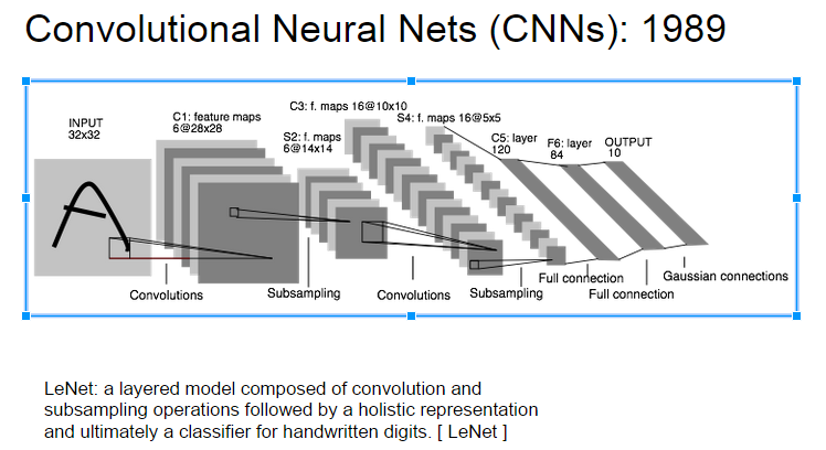
下面部分参考 Deep Learning（深度学习）学习笔记整理系列之（七）

LeNet中每个层有多个Feature Map，每个Feature Map通过一种卷积滤波器提取输入的一种特征，然后每个Feature Map有多个神经元

C1层是一个卷积层（为什么是卷积？卷积运算一个重要的特点就是，通过卷积运算，可以使原信号特征增强，并且降低噪音），由6个特征图Feature Map构成。特征图中每个神经元与输入中5*5的邻域相连。特征图的大小为28*28（28=32-5+1），这样能防止输入的连接掉到边界之外（是为了BP反馈时的计算，不致梯度损失，个人见解）。C1有156个可训练参数（每个滤波器5*5=25个unit参数和一个bias参数，一共6个滤波器，共(5*5+1)*6=156个参数），共156*(28*28)=122,304个连接。

S2层是一个下采样层（为什么是下采样？利用图像局部相关性的原理，对图像进行子抽样，可以减少数据处理量同时保留有用信息），有6个14*14的特征图。特征图中的每个单元与C1中相对应特征图的2*2邻域相连接。S2层每个单元的4个输入相加，乘以一个可训练参数，再加上一个可训练偏置。结果通过sigmoid函数计算。可训练系数和偏置控制着sigmoid函数的非线性程度。如果系数比较小，那么运算近似于线性运算，亚采样相当于模糊图像。如果系数比较大，根据偏置的大小亚采样可以被看成是有噪声的“或”运算或者有噪声的“与”运算。每个单元的2*2感受野并不重叠，因此S2中每个特征图的大小是C1中特征图大小的1/4（行和列各1/2）。S2层有12个可训练参数和5880个连接。

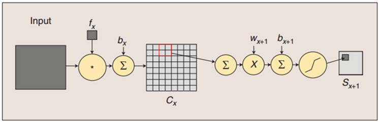
图：卷积和子采样过程：卷积过程包括：用一个可训练的滤波器fx去卷积一个输入的图像（第一阶段是输入的图像，后面的阶段就是卷积特征map了），然后加一个偏置bx，得到卷积层Cx。子采样过程包括：每邻域四个像素求和变为一个像素，然后通过标量Wx+1加权，再增加偏置bx+1，然后通过一个sigmoid激活函数，产生一个大概缩小四倍的特征映射图Sx+1。

所以从一个平面到下一个平面的映射可以看作是作卷积运算，S层可看作是模糊滤波器，起到二次特征提取的作用。隐层与隐层之间空间分辨率递减，而每层所含的平面数递增，这样可用于检测更多的特征信息。

C3层也是一个卷积层，它同样通过5x5的卷积核去卷积层S2，然后得到feature map就只有10x10个神经元，但是它有16种不同的卷积核，所以就存在16个feature map了。这里需要注意的一点是：C3中的每个feature map是连接到S2中的所有6个或者几个feature map的，表示本层的feature map是上一层提取到的feature map的不同组合（这个做法也并不是唯一的）。（这里是组合，就像之前聊到的人的视觉系统一样，底层的结构构成上层更抽象的结构，例如边缘构成形状或者目标的部分）。

S4层是一个下采样层，由16个5*5大小的特征图构成。特征图中的每个单元与C3中相应特征图的2*2邻域相连接，跟C1和S2之间的连接一样。S4层有32个可训练参数（每个特征图1个因子和一个偏置）和2000个连接。

C5层是一个卷积层，有120个特征图。每个单元与S4层的全部16个单元的5*5邻域相连。由于S4层特征图的大小也为5*5（同滤波器一样），故C5特征图的大小为1*1：这构成了S4和C5之间的全连接。之所以仍将C5标示为卷积层而非全相联层，是因为如果LeNet-5的输入变大，而其他的保持不变，那么此时特征图的维数就会比1*1大。C5层有48120个可训练连接。

F6层有84个单元（之所以选这个数字的原因来自于输出层的设计），与C5层全相连。有10164个可训练参数。如同经典神经网络，F6层计算输入向量和权重向量之间的点积，再加上一个偏置。然后将其传递给sigmoid函数产生单元i的一个状态。

最后，输出层由欧式径向基函数（Euclidean Radial Basis Function）单元组成，每类一个单元，每个有84个输入。换句话说，每个输出RBF单元计算输入向量和参数向量之间的欧式距离。输入离参数向量越远，RBF输出的越大。一个RBF输出可以被理解为衡量输入模式和与RBF相关联类的一个模型的匹配程度的惩罚项。用概率术语来说，RBF输出可以被理解为F6层配置空间的高斯分布的负log-likelihood。给定一个输入模式，损失函数应能使得F6的配置与RBF参数向量（即模式的期望分类）足够接近。这些单元的参数是人工选取并保持固定的（至少初始时候如此）。这些参数向量的成分被设为-1或1。虽然这些参数可以以-1和1等概率的方式任选，或者构成一个纠错码，但是被设计成一个相应字符类的7*12大小（即84）的格式化图片。这种表示对识别单独的数字不是很有用，但是对识别可打印ASCII集中的字符串很有用。

使用这种分布编码而非更常用的“1 of N”编码用于产生输出的另一个原因是，当类别比较大的时候，非分布编码的效果比较差。原因是大多数时间非分布编码的输出必须为0。这使得用sigmoid单元很难实现。另一个原因是分类器不仅用于识别字母，也用于拒绝非字母。使用分布编码的RBF更适合该目标。因为与sigmoid不同，他们在输入空间的较好限制的区域内兴奋，而非典型模式更容易落到外边。

RBF参数向量起着F6层目标向量的角色。需要指出这些向量的成分是+1或-1，这正好在F6 sigmoid的范围内，因此可以防止sigmoid函数饱和。实际上，+1和-1是sigmoid函数的最大弯曲的点处。这使得F6单元运行在最大非线性范围内。必须避免sigmoid函数的饱和，因为这将会导致损失函数较慢的收敛和病态问题。

Define the MNIST Network

This section explains the lenet_train_test.prototxt model definition that specifies(说明) the LeNet model for MNIST handwritten digit classification. We assume that you are familiar with
4000
Google Protobuf, and assume that you have read the protobuf definitions used by Caffe, which can be found at $CAFFE_ROOT/src/caffe/proto/caffe.proto.

Google Protocol Buffer 的使用和原理

Protocol Buffers (简称 Protobuf) 是一种轻便高效的结构化数据存储格式，可以用于结构化数据串行化，很适合做数据存储或 RPC 数据交换格式。它可用于通讯协议、数据存储等领域的语言无关、平台无关、可扩展的序列化结构数据格式。目前提供了 C++、Java、Python 三种语言的 API。

Specifically, we will write a caffe::NetParameter protobuf. We will start by giving the network a name:

name: "LeNet" //设置网络的名称

Writing the Data Layer

Currently, we will read the MNIST data from the lmdb we created earlier in the demo. This is defined by a data layer:

lmdb简介

原文链接：http://www.jianshu.com/p/yzFf8j

lmdb是openLDAP项目开发的嵌入式（作为一个库嵌入到宿主程序）存储引擎。其主要特性有：

基于文件映射IO（mmap）

基于B+树的key-value接口

基于MVCC（Multi Version Concurrent Control）的事务处理

类bdb（berkeley db）的api

/*数据层*/
layer {
name: "mnist"  //输入层的名字
type: "Data"   //输入层的类型
transform_param { //需要将输入像素灰度归一化到[0,1），故用1/256
scale: 0.00390625
}
data_param {
source: "mnist_train_lmdb" //从mnist_train_lmdb中读取数据
backend: LMDB //(暂时不知道意义）
batch_size: 64 //批次为64，即一次处理64条数据
}
top: "data" //此层后面连接data和label Blob空间
top: "label"
}

Specifically, this layer has name mnist, type data, and it reads the data from the given lmdb source. We will use a batch(脚本) size of 64, and scale the incoming pixels so that they are in the range [0,1). Why 0.00390625? It is 1 divided by 256. And finally, this layer produces two blobs, one is the data blob, and one is the label blob.

-

Writing the Convolution Layer

Let’s define the first convolution layer:

layer {
name: "conv1" //卷积层名字
type: "Convolution" //卷积层类型
param { lr_mult: 1 } //weight的学习率
param { lr_mult: 2 } //bias的学习率
convolution_param {  //卷积层参数
num_output: 20  //输出单元数目
kernel_size: 5  //卷积核大小为5*5
stride: 1  //步长为1
weight_filler {  //网络允许用随机值初始化权重和偏置
type: "xavier"  //xavier算法自动确定基于输入和输出神经元数量的初始规模
}
bias_filler {  //偏置值初始化为常数，默认为0
type: "constant"
}
}
bottom: "data"  //此层前面使用data后面生成conv1的blob空间
top: "conv1"
}

This layer takes the data blob (it is provided by the data layer), and produces the conv1 layer. It produces outputs of 20 channels, with the convolutional kernel size 5 and carried out with stride 1.

lr_mults are the learning rate adjustments for the layer’s learnable parameters. In this case, we will set the weight learning rate to be the same as the learning rate given by the solver during runtime, and the bias learning rate to be twice as large as that - this usually leads to better convergence rates.

即设置权值学习率与solver中提供的学习率相同，并设置偏置学习率为权值学习率的两倍，这种设置可以保证较好的收敛速度。

Writing the Pooling Layer

layer {
name: "pool1"
type: "Pooling"
pooling_param {
kernel_size: 2
stride: 2
pool: MAX  //池化方式为MAX
}
bottom: "conv1"
top: "pool1"
}

This says we will perform max pooling with a pool kernel size 2 and a stride of 2 (so no overlapping between neighboring pooling regions).

Writing the Fully Connected Layer

Writing a fully connected layer is also simple:

layer {
name: "ip1"
type: "InnerProduct"  //全连接层，与卷积层相似
param { lr_mult: 1 }
param { lr_mult: 2 }
inner_product_param {
num_output: 500  //输出500个节点，据说一定范围内此值越大正确率越高（待检测）
weight_filler {
type: "xavier"
}
bias_filler {
type: "constant"
}
}
bottom: "pool2"
top: "ip1"
}

This defines a fully connected layer (known in Caffe as an InnerProduct layer) with 500 outputs.

Writing the ReLU Layer

A ReLU Layer is also simple:

layer {  //ReLU线性纠正函数取代sigmod函数来激活神经元
name: "relu1"
type: "ReLU"  //ReLU为非线性变化层 max( 0 ,x )
bottom: "ip1"
top: "ip1"
}

Since ReLU is an element-wise operation（元素级操作）, we can do in-place operations（现场激活操作） to save some memory. This is achieved by simply giving the same name to the bottom and top blobs. Of course, do NOT use duplicated blob names for other layer types!

由于ReLU为元素级操作，因此我们可以利用现场激活来节省内存，即利用bottom与top同名来实现，但此种方式不可在其他类型 层中使用。

After the ReLU layer, we will write another innerproduct layer:

layer {
name: "ip2"
type: "InnerProduct"
param { lr_mult: 1 }
param { lr_mult: 2 }
inner_product_param {
num_output: 10
weight_filler {
type: "xavier"
}
bias_filler {
type: "constant"
}
}
bottom: "ip1"
top: "ip2"
}

Writing the Loss Layer

Finally, we will write the loss!

layer {
name: "loss"
type: "SoftmaxWithLoss"
bottom: "ip2"
bottom: "label"
}

The softmax_loss layer implements both the softmax and the multinomial logistic loss (that saves time and improves numerical stability). It takes two blobs, the first one being the prediction and the second one being the label provided by the data layer (remember it?). It does not produce any outputs - all it does is to compute the loss function value, report it when backpropagation starts, and initiates the gradient with respect to ip2. This is where all magic starts.

Define the MNIST Solver

/*训练/测试网络的定义（即上文部分）*/
net: "examples/mnist/lenet_train_test.prototxt"
/*test_iter: 在测试的时候，需要迭代的次数，即test_iter* batch_size（测试集的）=测试集的大小，测试集的batch_size可以在prototx文件里设置。例如，在mnist中，设batch_size=100,test_iter=100,最后测试100*100张图片*/
test_iter: 100
/*test_interval:训练的时候，每迭代500次就进行一次误差测试。*/
test_interval: 500
/*学习率，动量，权重递减*/
base_lr: 0.01
momentum: 0.9
weight_decay: 0.0005
/*学习政策，cifar10类用固定学习率，imagenet用每步递减学习率
lr_policy: "inv"
gamma: 0.0001
power: 0.75
/*每迭代100次显示一次*/
display: 100
/*最大迭代次数*/
max_iter: 10000
/*每5000次迭代存储一次数据到电脑，名称为"lenet"
snapshot: 5000
snapshot_prefix: "examples/mnist/lenet"
# solver 模式: CPU or GPU
solver_mode: GPU

Training and Testing the Model

Training the model is simple after you have written the network definition protobuf and solver protobuf files. Simply run train_lenet.sh, or the following command directly:

cd $CAFFE_ROOT
./examples/mnist/train_lenet.sh //注意要在CAFFE_ROOT目录下面运行

train_lenet.sh is a simple script（简单脚本）, but here is a quick explanation: the main tool for training is caffe with action train and the solver protobuf text file as its argument.

Training and Testing the Model

For each training iteration, lr is the learning rate of that iteration, and loss is the training function. For the output of the testing phase, score 0 is the accuracy, and score 1 is the testing loss function.

I1203 solver.cpp:84] Testing net
I1203 solver.cpp:111] Test score #0: 0.9785
I1203 solver.cpp:111] Test score #1: 0.0606671