RNN-RBM 网络架构及程序解读
2016-03-17 12:59
627 查看
对RNN-RBM代码的部分解析:
<span style="font-size:18px;">from __future__ import print_function
import glob
import os
import sys
import numpy
try:
import pylab
except ImportError:
print ("pylab isn't available. If you use its functionality, it will crash.")
print("It can be installed with 'pip install -q Pillow'")
from midi.utils import midiread, midiwrite
import theano
import theano.tensor as T
from theano.tensor.shared_randomstreams import RandomStreams
#Don't use a python long as this don't work on 32 bits computers.
numpy.random.seed(0xbeef)
rng = RandomStreams(seed=numpy.random.randint(1 << 30))
theano.config.warn.subtensor_merge_bug = False
def build_rbm(v, W, bv, bh, k):
'''Construct a k-step Gibbs chain starting at v for an RBM.
v : Theano vector or matrix
If a matrix, multiple chains will be run in parallel (batch).
W : Theano matrix
Weight matrix of the RBM.
bv : Theano vector
Visible bias vector of the RBM.
bh : Theano vector
Hidden bias vector of the RBM.
k : scalar or Theano scalar
Length of the Gibbs chain.
Return a (v_sample, cost, monitor, updates) tuple:
v_sample : Theano vector or matrix with the same shape as `v`
Corresponds to the generated sample(s).
cost : Theano scalar
Expression whose gradient with respect to W, bv, bh is the CD-k
approximation to the log-likelihood of `v` (training example) under the
RBM. The cost is averaged in the batch case.
monitor: Theano scalar
Pseudo log-likelihood (also averaged in the batch case).
updates: dictionary of Theano variable -> Theano variable
The `updates` object returned by scan.'''
def gibbs_step(v):
mean_h = T.nnet.sigmoid(T.dot(v, W) + bh)
h = rng.binomial(size=mean_h.shape, n=1, p=mean_h,
dtype=theano.config.floatX)
mean_v = T.nnet.sigmoid(T.dot(h, W.T) + bv)
v = rng.binomial(size=mean_v.shape, n=1, p=mean_v,
dtype=theano.config.floatX)
return mean_v, v
chain, updates = theano.scan(lambda v: gibbs_step(v)[1], outputs_info=[v],
n_steps=k)
# -1表示从后边开始取值。
v_sample = chain[-1]
mean_v = gibbs_step(v_sample)[0]
monitor = T.xlogx.xlogy0(v, mean_v) + T.xlogx.xlogy0(1 - v, 1 - mean_v)
monitor = monitor.sum() / v.shape[0]
def free_energy(v):
return -(v * bv).sum() - T.log(1 + T.exp(T.dot(v, W) + bh)).sum()
cost = (free_energy(v) - free_energy(v_sample)) / v.shape[0]
return v_sample, cost, monitor, updates</span>
简单介绍下RBM网络,因为deep learning中的一个重要网络结构DBN就可以由RBM网络叠加而成,所以对RBM的理解有利于我们对DBN算法以及deep learning算法的进一步理解。Deep learning是从06年开始火得,得益于大牛Hinton的文章,不过这位大牛的文章比较晦涩难懂,公式太多,对于我这种菜鸟级别来说读懂它的paper压力太大。纵观大部分介绍RBM的paper,都会提到能量函数。因此有必要先了解下能量函数的概念。参考网页http://202.197.191.225:8080/30/text/chapter06/6_2t24.htm关于能量函数的介绍:
一个事物有相应的稳态,如在一个碗内的小球会停留在碗底,即使受到扰动偏离了碗底,在扰动消失后,它会回到碗底。学过物理的人都知道,稳态是它势能最低的状态。因此稳态对应与某一种能量的最低状态。将这种概念引用到Hopfield网络中去,Hopfield构造了一种能量函数的定义。这是他所作的一大贡献。引进能量函数概念可以进一步加深对这一类动力系统性质的认识,可以把求稳态变成一个求极值与优化的问题,从而为Hopfield网络找到一个解优化问题的应用。
下面来看看RBM网络,其结构图如下所示:

可以看到RBM网络共有2层,其中第一层称为可视层,一般来说是输入层,另一层是隐含层,也就是我们一般指的特征提取层。在一般的文章中,都把这2层的节点看做是二值的,也就是只能取0或1,当然了,RBM中节点是可以取实数值的,这里取二值只是为了更好的解释各种公式而已。在前面一系列的博文中可以知道,我们设计一个网络结构后,接下来就应该想方设法来求解网络中的参数值。而这又一般是通过最小化损失函数值来解得的,比如在autoencoder中是通过重构值和输入值之间的误差作为损失函数(当然了,一般都会对参数进行规制化的);在logistic回归中损失函数是与输出值和样本标注值的差有关。那么在RBM网络中,我们的损失函数的表达式是什么呢,损失函数的偏导函数又该怎么求呢?
在了解这个问题之前,我们还是先从能量函数出发。针对RBM模型而言,输入v向量和隐含层输出向量h之间的能量函数值为:

而这2者之间的联合概率为:

其中Z是归一化因子,其值为:

这里为了习惯,把输入v改成函数的自变量x,则关于x的概率分布函数为:

令一个中间变量F(x)为:

则x的概率分布可以重新写为:

这时候它的偏导函数取负后为:

从上面能量函数的抽象介绍中可以看出,如果要使系统(这里即指RBM网络)达到稳定,则应该是系统的能量值最小,由上面的公式可知,要使能量E最小,应该使F(x)最小,也就是要使P(x)最大。因此此时的损失函数可以看做是-P(x),且求导时需要是加上负号的。
另外在图RBM中,可以很容易得到下面的概率值公式:

此时的F(v)为(也就是F(x)):

这个函数也被称做是自由能量函数。另外经过一些列的理论推导,可以求出损失函数的偏导函数公式为:

很明显,我们这里是吧-P(v)当成了损失函数了。那么为什么要用随机采用来得到数据呢,我们不是都有训练样本数据了么?其实这个问题我也一直没弄明白。在看过一些简单的RBM代码后,暂时只能这么理解:在上面文章最后的求偏导公式里,是两个数的减法,按照一般paper上所讲,这个被减数等于输入样本数据的自由能量函数期望值,而减数是模型产生样本数据的自由能量函数期望值。而这个模型样本数据就是利用Gibbs采样获得的,大概就是用原始的数据v输入到网络,计算输出h(1),然后又反推v(1),继续计算h(2),…,当最后反推出的v(k)和k比较接近时停止,这个时候的v(k)就是模型数据样本了。
2. RNN-RBM的定义:
2.1 RTRBM结构
首先我们以RTRBM(RNNRBM简化版,由Sutskever于08年提出)介入。以下是RTRBM的结构:
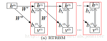
图中每一个红框框住了一个RBM,h是hidden states,v是visible nodes,比如表示为某一时刻的语音等(但实际上为了增加维度有些工作会把v(t)扩展为前后共n帧data的value),双向箭头表示h和v生成的条件概率,即:
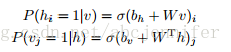
(1)
其中σ是sigmoid函数。
对于每个时刻的RBM,v和h的联合概率分布为:
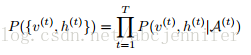
(2)
其中A(t)=
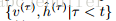
,即所有t时刻之前的{v,h}集合。
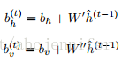
此外对于RTRBM,可以理解为每个时刻可以由上一时刻的状态h(t-1)对该时刻产生影响(通过W'和W''),然后通过RBM得到一个(h(t),v(t))稳态。由于每一个参数都和上一时刻的参数有关,我们可以认为只有bias项是受hidden影响的,这样效果是一样的,即:
(2)
2.2 RNN-RBM网络架构
看到了RTRBM这个结构,bengio他们就想了,RTRBM结构里hidden layer描述的是visible的条件概率分布,只能保存暂时的信息(他应该指的是达到稳态后),那我能不能把这些rbm里的hidden layer用RNN代替?于是就冒出了RNN-RBM:
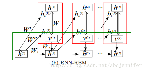
其中每个红框依然框住一个RBM,而下面绿框就表示了一个按时间展开了的RNN。这样设计的好处是把hiddenlayer分离了,一部分(h)只用于表示当前RBM的稳态state,另一部分(h^)表示RNN里的hidden节点。
PS: 关于RNN的网络结构:v(visible),u(internal units),h(hidden)
边:v-u, u-v, v-h(双向边,==h-v), u-h, u-u(实际上是环,只不过时序模型中unfold成u^t-u^{t+1})
这些边在不同level(sequence的不同时刻)是共享权值滴。
所以我们实际上要优化的参数就是上面的5个weight matrix加bv,bh,bu
2.3 RNN-RBM 的训练
1. 由
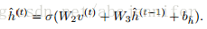
计算h^
2. 由(2)计算bh, bv,并根据k-step block gibbs采样得到v(t)
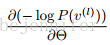
3. 通过NLL的cost
对RBM里的参数(W,
bh, bv)进行求导并更新
4. 估计RNN参数(W2, W3, bh^)并进行更新
<span style="font-size:18px;">from __future__ import print_function
import glob
import os
import sys
import numpy
try:
import pylab
except ImportError:
print ("pylab isn't available. If you use its functionality, it will crash.")
print("It can be installed with 'pip install -q Pillow'")
from midi.utils import midiread, midiwrite
import theano
import theano.tensor as T
from theano.tensor.shared_randomstreams import RandomStreams
#Don't use a python long as this don't work on 32 bits computers.
numpy.random.seed(0xbeef)
rng = RandomStreams(seed=numpy.random.randint(1 << 30))
theano.config.warn.subtensor_merge_bug = False
def build_rbm(v, W, bv, bh, k):
'''Construct a k-step Gibbs chain starting at v for an RBM.
v : Theano vector or matrix
If a matrix, multiple chains will be run in parallel (batch).
W : Theano matrix
Weight matrix of the RBM.
bv : Theano vector
Visible bias vector of the RBM.
bh : Theano vector
Hidden bias vector of the RBM.
k : scalar or Theano scalar
Length of the Gibbs chain.
Return a (v_sample, cost, monitor, updates) tuple:
v_sample : Theano vector or matrix with the same shape as `v`
Corresponds to the generated sample(s).
cost : Theano scalar
Expression whose gradient with respect to W, bv, bh is the CD-k
approximation to the log-likelihood of `v` (training example) under the
RBM. The cost is averaged in the batch case.
monitor: Theano scalar
Pseudo log-likelihood (also averaged in the batch case).
updates: dictionary of Theano variable -> Theano variable
The `updates` object returned by scan.'''
def gibbs_step(v):
mean_h = T.nnet.sigmoid(T.dot(v, W) + bh)
h = rng.binomial(size=mean_h.shape, n=1, p=mean_h,
dtype=theano.config.floatX)
mean_v = T.nnet.sigmoid(T.dot(h, W.T) + bv)
v = rng.binomial(size=mean_v.shape, n=1, p=mean_v,
dtype=theano.config.floatX)
return mean_v, v
chain, updates = theano.scan(lambda v: gibbs_step(v)[1], outputs_info=[v],
n_steps=k)
# -1表示从后边开始取值。
v_sample = chain[-1]
mean_v = gibbs_step(v_sample)[0]
monitor = T.xlogx.xlogy0(v, mean_v) + T.xlogx.xlogy0(1 - v, 1 - mean_v)
monitor = monitor.sum() / v.shape[0]
def free_energy(v):
return -(v * bv).sum() - T.log(1 + T.exp(T.dot(v, W) + bh)).sum()
cost = (free_energy(v) - free_energy(v_sample)) / v.shape[0]
return v_sample, cost, monitor, updates</span>
简单介绍下RBM网络,因为deep learning中的一个重要网络结构DBN就可以由RBM网络叠加而成,所以对RBM的理解有利于我们对DBN算法以及deep learning算法的进一步理解。Deep learning是从06年开始火得,得益于大牛Hinton的文章,不过这位大牛的文章比较晦涩难懂,公式太多,对于我这种菜鸟级别来说读懂它的paper压力太大。纵观大部分介绍RBM的paper,都会提到能量函数。因此有必要先了解下能量函数的概念。参考网页http://202.197.191.225:8080/30/text/chapter06/6_2t24.htm关于能量函数的介绍:
一个事物有相应的稳态,如在一个碗内的小球会停留在碗底,即使受到扰动偏离了碗底,在扰动消失后,它会回到碗底。学过物理的人都知道,稳态是它势能最低的状态。因此稳态对应与某一种能量的最低状态。将这种概念引用到Hopfield网络中去,Hopfield构造了一种能量函数的定义。这是他所作的一大贡献。引进能量函数概念可以进一步加深对这一类动力系统性质的认识,可以把求稳态变成一个求极值与优化的问题,从而为Hopfield网络找到一个解优化问题的应用。
下面来看看RBM网络,其结构图如下所示:
可以看到RBM网络共有2层,其中第一层称为可视层,一般来说是输入层,另一层是隐含层,也就是我们一般指的特征提取层。在一般的文章中,都把这2层的节点看做是二值的,也就是只能取0或1,当然了,RBM中节点是可以取实数值的,这里取二值只是为了更好的解释各种公式而已。在前面一系列的博文中可以知道,我们设计一个网络结构后,接下来就应该想方设法来求解网络中的参数值。而这又一般是通过最小化损失函数值来解得的,比如在autoencoder中是通过重构值和输入值之间的误差作为损失函数(当然了,一般都会对参数进行规制化的);在logistic回归中损失函数是与输出值和样本标注值的差有关。那么在RBM网络中,我们的损失函数的表达式是什么呢,损失函数的偏导函数又该怎么求呢?
在了解这个问题之前,我们还是先从能量函数出发。针对RBM模型而言,输入v向量和隐含层输出向量h之间的能量函数值为:
而这2者之间的联合概率为:
其中Z是归一化因子,其值为:
这里为了习惯,把输入v改成函数的自变量x,则关于x的概率分布函数为:
令一个中间变量F(x)为:
则x的概率分布可以重新写为:
这时候它的偏导函数取负后为:
从上面能量函数的抽象介绍中可以看出,如果要使系统(这里即指RBM网络)达到稳定,则应该是系统的能量值最小,由上面的公式可知,要使能量E最小,应该使F(x)最小,也就是要使P(x)最大。因此此时的损失函数可以看做是-P(x),且求导时需要是加上负号的。
另外在图RBM中,可以很容易得到下面的概率值公式:
此时的F(v)为(也就是F(x)):
这个函数也被称做是自由能量函数。另外经过一些列的理论推导,可以求出损失函数的偏导函数公式为:
很明显,我们这里是吧-P(v)当成了损失函数了。那么为什么要用随机采用来得到数据呢,我们不是都有训练样本数据了么?其实这个问题我也一直没弄明白。在看过一些简单的RBM代码后,暂时只能这么理解:在上面文章最后的求偏导公式里,是两个数的减法,按照一般paper上所讲,这个被减数等于输入样本数据的自由能量函数期望值,而减数是模型产生样本数据的自由能量函数期望值。而这个模型样本数据就是利用Gibbs采样获得的,大概就是用原始的数据v输入到网络,计算输出h(1),然后又反推v(1),继续计算h(2),…,当最后反推出的v(k)和k比较接近时停止,这个时候的v(k)就是模型数据样本了。
<span style="font-size:18px;">def shared_normal(num_rows, num_cols, scale=1):
'''Initialize a matrix shared variable with normally distributed
elements.'''
return theano.shared(numpy.random.normal(
scale=scale, size=(num_rows, num_cols)).astype(theano.config.floatX))

def shared_zeros(*shape):
'''Initialize a vector shared variable with zero elements.'''
return theano.shared(numpy.zeros(shape, dtype=theano.config.floatX))</span>
<span style="font-size:18px;">def build_rnnrbm(n_visible, n_hidden, n_hidden_recurrent):
'''Construct a symbolic RNN-RBM and initialize parameters.

n_visible : integer
Number of visible units.
n_hidden : integer
Number of hidden units of the conditional RBMs.
n_hidden_recurrent : integer
Number of hidden units of the RNN.

Return a (v, v_sample, cost, monitor, params, updates_train, v_t,
updates_generate) tuple:

v : Theano matrix
Symbolic variable holding an input sequence (used during training)
v_sample : Theano matrix
Symbolic variable holding the negative particles for CD log-likelihood
gradient estimation (used during training)
cost : Theano scalar
Expression whose gradient (considering v_sample constant) corresponds
to the LL gradient of the RNN-RBM (used during training)
monitor : Theano scalar
Frame-level pseudo-likelihood (useful for monitoring during training)
params : tuple of Theano shared variables
The parameters of the model to be optimized during training.
updates_train : dictionary of Theano variable -> Theano variable
Update object that should be passed to theano.function when compiling
the training function.
v_t : Theano matrix
Symbolic variable holding a generated sequence (used during sampling)
updates_generate : dictionary of Theano variable -> Theano variable
Update object that should be passed to theano.function when compiling
the generation function.'''

W = shared_normal(n_visible, n_hidden, 0.01)
bv = shared_zeros(n_visible)
bh = shared_zeros(n_hidden)
Wuh = shared_normal(n_hidden_recurrent, n_hidden, 0.0001)
Wuv = shared_normal(n_hidden_recurrent, n_visible, 0.0001)
Wvu = shared_normal(n_visible, n_hidden_recurrent, 0.0001)
Wuu = shared_normal(n_hidden_recurrent, n_hidden_recurrent, 0.0001)
bu = shared_zeros(n_hidden_recurrent)

params = W, bv, bh, Wuh, Wuv, Wvu, Wuu, bu  # learned parameters as shared
# variables

v = T.matrix()  # a training sequence
u0 = T.zeros((n_hidden_recurrent,))  # initial value for the RNN hidden
# units

# If `v_t` is given, deterministic recurrence to compute the variable
# biases bv_t, bh_t at each time step. If `v_t` is None, same recurrence
# but with a separate Gibbs chain at each time step to sample (generate)
# from the RNN-RBM. The resulting sample v_t is returned in order to be
# passed down to the sequence history.
def recurrence(v_t, u_tm1):
bv_t = bv + T.dot(u_tm1, Wuv)
bh_t = bh + T.dot(u_tm1, Wuh)
generate = v_t is None
if generate:
v_t, _, _, updates = build_rbm(T.zeros((n_visible,)), W, bv_t,
bh_t, k=25)
u_t = T.tanh(bu + T.dot(v_t, Wvu) + T.dot(u_tm1, Wuu))
return ([v_t, u_t], updates) if generate else [u_t, bv_t, bh_t]

# For training, the deterministic recurrence is used to compute all the
# {bv_t, bh_t, 1 <= t <= T} given v. Conditional RBMs can then be trained
# in batches using those parameters.
(u_t, bv_t, bh_t), updates_train = theano.scan(
lambda v_t, u_tm1, *_: recurrence(v_t, u_tm1),
sequences=v, outputs_info=[u0, None, None], non_sequences=params)
v_sample, cost, monitor, updates_rbm = build_rbm(v, W, bv_t[:], bh_t[:],
k=15)
updates_train.update(updates_rbm)

# symbolic loop for sequence generation
(v_t, u_t), updates_generate = theano.scan(
lambda u_tm1, *_: recurrence(None, u_tm1),
outputs_info=[None, u0], non_sequences=params, n_steps=200)

return (v, v_sample, cost, monitor, params, updates_train, v_t,
updates_generate)</span>
2. RNN-RBM的定义:
2.1 RTRBM结构
首先我们以RTRBM(RNNRBM简化版,由Sutskever于08年提出)介入。以下是RTRBM的结构:
图中每一个红框框住了一个RBM,h是hidden states,v是visible nodes,比如表示为某一时刻的语音等(但实际上为了增加维度有些工作会把v(t)扩展为前后共n帧data的value),双向箭头表示h和v生成的条件概率,即:
(1)
其中σ是sigmoid函数。
对于每个时刻的RBM,v和h的联合概率分布为:
(2)
其中A(t)=
,即所有t时刻之前的{v,h}集合。
此外对于RTRBM,可以理解为每个时刻可以由上一时刻的状态h(t-1)对该时刻产生影响(通过W'和W''),然后通过RBM得到一个(h(t),v(t))稳态。由于每一个参数都和上一时刻的参数有关,我们可以认为只有bias项是受hidden影响的,这样效果是一样的,即:
(2)
2.2 RNN-RBM网络架构
看到了RTRBM这个结构,bengio他们就想了,RTRBM结构里hidden layer描述的是visible的条件概率分布,只能保存暂时的信息(他应该指的是达到稳态后),那我能不能把这些rbm里的hidden layer用RNN代替?于是就冒出了RNN-RBM:
其中每个红框依然框住一个RBM,而下面绿框就表示了一个按时间展开了的RNN。这样设计的好处是把hiddenlayer分离了,一部分(h)只用于表示当前RBM的稳态state,另一部分(h^)表示RNN里的hidden节点。
PS: 关于RNN的网络结构:v(visible),u(internal units),h(hidden)
边:v-u, u-v, v-h(双向边,==h-v), u-h, u-u(实际上是环,只不过时序模型中unfold成u^t-u^{t+1})
这些边在不同level(sequence的不同时刻)是共享权值滴。
所以我们实际上要优化的参数就是上面的5个weight matrix加bv,bh,bu
2.3 RNN-RBM 的训练
1. 由
计算h^
2. 由(2)计算bh, bv,并根据k-step block gibbs采样得到v(t)
3. 通过NLL的cost
对RBM里的参数(W,
bh, bv)进行求导并更新
4. 估计RNN参数(W2, W3, bh^)并进行更新
<span style="font-size:18px;">class RnnRbm:
'''Simple class to train an RNN-RBM from MIDI files and to generate sample
sequences.'''

def __init__(
self,
n_hidden=150,
n_hidden_recurrent=100,
lr=0.001,
r=(21, 109),
dt=0.3
):
'''Constructs and compiles Theano functions for training and sequence
generation.

n_hidden : integer
Number of hidden units of the conditional RBMs.
n_hidden_recurrent : integer
Number of hidden units of the RNN.
lr : float
Learning rate
r : (integer, integer) tuple
Specifies the pitch range of the piano-roll in MIDI note numbers,
including r[0] but not r[1], such that r[1]-r[0] is the number of
visible units of the RBM at a given time step. The default (21,
109) corresponds to the full range of piano (88 notes).
dt : float
Sampling period when converting the MIDI files into piano-rolls, or
equivalently the time difference between consecutive time steps.'''

self.r = r
self.dt = dt
(v, v_sample, cost, monitor, params, updates_train, v_t,
updates_generate) = build_rnnrbm(
r[1] - r[0],
n_hidden,
n_hidden_recurrent
)

gradient = T.grad(cost, params, consider_constant=[v_sample])
updates_train.update(
((p, p - lr * g) for p, g in zip(params, gradient))
)
self.train_function = theano.function(
[v],
monitor,
updates=updates_train
)
self.generate_function = theano.function(
[],
v_t,
updates=updates_generate
)

def train(self, files, batch_size=100, num_epochs=200):
'''Train the RNN-RBM via stochastic gradient descent (SGD) using MIDI
files converted to piano-rolls.

files : list of strings
List of MIDI files that will be loaded as piano-rolls for training.
batch_size : integer
Training sequences will be split into subsequences of at most this
size before applying the SGD updates.
num_epochs : integer
Number of epochs (pass over the training set) performed. The user
can safely interrupt training with Ctrl+C at any time.'''

assert len(files) > 0, 'Training set is empty!' \
' (did you download the data files?)'
dataset = [midiread(f, self.r,
self.dt).piano_roll.astype(theano.config.floatX)
for f in files]

try:
for epoch in range(num_epochs):
numpy.random.shuffle(dataset)
costs = []

for s, sequence in enumerate(dataset):
for i in range(0, len(sequence), batch_size):
cost = self.train_function(sequence[i:i + batch_size])
costs.append(cost)

print('Epoch %i/%i' % (epoch + 1, num_epochs))
print(numpy.mean(costs))
sys.stdout.flush()

except KeyboardInterrupt:
print('Interrupted by user.')

def generate(self, filename, show=True):
'''Generate a sample sequence, plot the resulting piano-roll and save
it as a MIDI file.

filename : string
A MIDI file will be created at this location.
show : boolean
If True, a piano-roll of the generated sequence will be shown.'''

piano_roll = self.generate_function()
midiwrite(filename, piano_roll, self.r, self.dt)
if show:
extent = (0, self.dt * len(piano_roll)) + self.r
pylab.figure()
pylab.imshow(piano_roll.T, origin='lower', aspect='auto',
interpolation='nearest', cmap=pylab.cm.gray_r,
extent=extent)
pylab.xlabel('time (s)')
pylab.ylabel('MIDI note number')
pylab.title('generated piano-roll')

def test_rnnrbm(batch_size=100, num_epochs=200):
model = RnnRbm()
#re = os.path.join(os.path.split(os.path.dirname(__file__))[0],
#                 'data', 'Nottingham', 'train', '*.mid')

re = os.path.join('data', 'Nottingham', 'train', '*.mid')
model.train(glob.glob(re),
batch_size=batch_size, num_epochs=num_epochs)
return model

if __name__ == '__main__':
model = test_rnnrbm()
model.generate('sample1.mid')
model.generate('sample2.mid')
pylab.show()</span>

相关文章推荐
- Restricted Boltzmann Machine 受玻尔兹曼机与DBM深度信念网络
- RBM学习算法
- RNN的通俗讲解(初级篇)
- RBM学习笔记
- char-cnn+torch+ubuntu14.04(RNN)
- 『RNN 监督序列标注』笔记-第一/二章 监督序列标注
- 『RNN 监督序列标注』笔记-第三章 神经网络
- 『RNN 监督序列标注』笔记-第四章 LSTM(Long Short-Term Memory)
- DBN爬坑记之RBM
- LSTM模型理论总结(产生、发展和性能等)
- RNN学习笔记(一)-简介及BPTT RTRL及Hybrid(FP/BPTT)算法
- RNN学习笔记(二)-Gradient Analysis
- Yusuke Sugomori 的 C 语言 Deep Learning 程序解读
- 受限玻尔兹曼机(RBM)学习笔记(一)预备知识
- 受限玻尔兹曼机(RBM)学习笔记(二)网络结构
- 受限玻尔兹曼机(RBM)学习笔记(三)能量函数和概率分布
- 受限玻尔兹曼机(RBM)学习笔记(四)对数似然函数
- 受限玻尔兹曼机(RBM)学习笔记(五)梯度计算公式
- 受限玻尔兹曼机(RBM)学习笔记(六)对比散度算法
- 受限玻尔兹曼机(RBM)学习笔记(七)RBM 训练算法