用Python做数据分析
2016-03-15 14:54
447 查看
背景
数据分析类问题在一些学术论坛上很常见。常用的软件SPSS, Matlab, Excel等都不是开源自由免费的。Python的好处主要是免费开源,不好用的话还可以ZB。转载下,半转半译,自己也是学习。来自下面的链接(我对代码稍微修改了下,图文跟代码可能不符):
Linear Regression: The Code
Data analysis with Python
Linear Regression
linear regression was all about: you have data in the form of a matrix X where rows correspond to datapoints, and columns correspond to features, and a column vector Y of corresponding response values. We seek a β so that Xβ is as close to Y as possible.We saw that we can find the solution by solving the linear system XTXβ=XTY for β
(多元线性回归,总是可以归结为求关于β的通常是超定的线性方程组,最小二乘最常用Moore-Penrose广义逆(最稳健的求解方法,效率虽低,但这类似计算通常很快) β^=(XTX)+XTY).
To do this in Python will be very simple using
scipy.linalg! I have created an IPython notebook taking you through everything, which you can run interactively. 这里顺便能看到Python的另外一个好处,scipy里面集成了成熟的、常用的、经典的线性代数计算的工具,免费开源而且好用。
Let’s begin by creating some data to model to get a feel for what we are doing. We’ll start with a linear function f, and add some Gaussian noise to make it a bit more realistic, then use linear regression to fit that data, and see how well we do compared with the true function f. 此处的例子,先给出一个斜率和截距确定的直线,然后在它的基础上随机取一系列x值并从小到大排序,然后对不同的x计算出直线上的y值,并给它添加一个均值和标准差固定的随机的高斯噪声或白噪声。然后,从一系列带有白噪声的这些点中,尝试用线性回归法拟合原来的直线;定义的第一个函数只是生成数据和模型的
#First get all the inclusions out of the way.
import numpy as np
from scipy import linalg
import random as rd
import matplotlib.pyplot as plt
def test_set(a,b, no_samples, intercept, slope, variance):
#First we grab some random x-values in the range [a,b].
X = [rd.uniform(a,b) for i in range(no_samples)]
#Sorting them seems to make the plots work better later on.
X.sort()
#Now we define our linear function that will underly our synthetic dataset: the true model.
def f(x):
return intercept + slope*x
#We create some y values to go with each x, given by f(x) plus a small perturbation by Gaussian noise.
Y = [f(x)+rd.gauss(0,variance) for x in X]
#Now we return these as numpy column vectors, as well as the points given by f without noise.
return [np.array([X]).T,np.array([Y]).T, map(f, X)]
Now let’s see what this looks like by plotting the data along with the graph of f. 显示所选取的直线、计算得到的添加了白噪声的离散点的散点图。
X,Y,f = test_set(a=0, b=5, no_samples=70, intercept=1, slope=3, variance=6)
fig, ax = plt.subplots()
ax.plot(X, Y, '.')
ax.plot(X, f)
plt.show()
This will look something like:
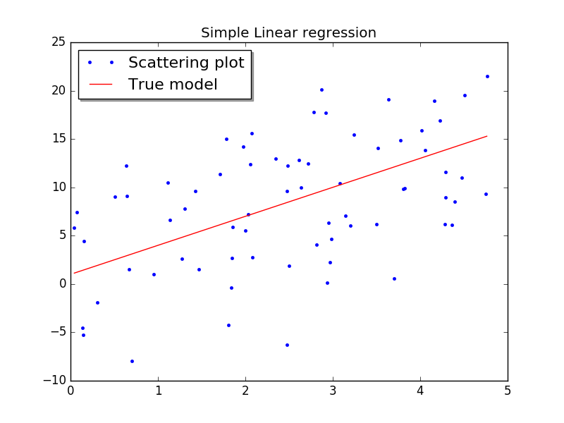
but of course yours will not look exactly the same because the data is generated randomly. The code for doing the linear regression is simplicity itself. 因为白噪声是通过伪随机数随机发生的,所以,不同的人操作的时候,看到的离散点的情况会不同;不过理论上应该也可以通过设定随机数发生器的初始状态,让每次的结果都一样。
def linear_regression(X, Y):
#solve linear system X^TXY = XB
beta=np.linalg.solve(X.T.dot(X),X.T.dot(Y))
return beta
Now we want to test it on our data, note that we want to add an extra column to X filled with ones, since if we just take a linear combination of X we will always go through the origin – we want an intercept term.
X = np.hstack((X, np.ones((X.shape[0], 1), dtype=X.dtype)))
beta=linear_regression(X, Y)
fig, ax = plt.subplots()
ax.plot(X[:,0], Y, '.', label="True model + noise")
ax.plot(X[:,0], f, '-', color='red', label="True model")
ax.plot(X[:,0], X.dot(beta), color='green',label="Fitted model")
legend = ax.legend(loc='lower right', shadow=True)
plt.show()
print "Fitted Slope = ", beta[0][0], "True Slope = 3"
print "Intercept =", beta[1][0], "True Intercept = 1"
Producing something like:
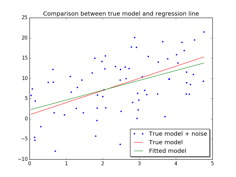
Well, the slope is not far off, but the intercept is wrong! This mostly comes from the noise we added,larger variance will mean poorer approximations to the true model, and more data will mean better approximations.If you run the code a couple of times, you will see quite a lot of variation. So maybe what we need to is try and quantify our uncertainty about the fit. We can do this by using bootstrapping as we discussed previously. 这里后面会用到的bootstrap中文翻译方法很多,一时也难以统一,而且这种统计方法在国内似乎也不够主流常用,早年的经典的概率统计之类的中文教科书很少提及,这也是没有统一的中文对应概念、近些年翻译五花八门的原因。不过我私下以为,统计工具使用的普及程度,基本上可以用来衡量一个国家在质量管理和控制方面的素质和水平。这些年我们的制造业都是在跟外企学习,培养了很多这方面的人才,这是国内大学教育反而做不到的。
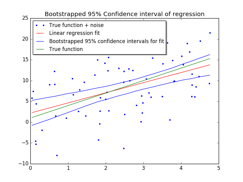
To get 95% condidence bounds for our fit, we will take a 1000 resamples of our data and fit each, then extract the quantiles from their predictions. 不过单纯对线性回归的95置信区间的计算来说, 增加取样并不是必须的(这种技巧在电子元件的行业里被一些国际企业用作产品标准制定和质量检测的依据; 现在看来,如果样本比较小,还应该加上bootstrapping技巧才更合适)
First we get the β for each resample.
betas=[]
N= X.shape[0]
for resample in range(1000):
index = [rd.choice(range(N)) for i in range(N)]
re_X=X[index,:]
betas.append(linear_regression(re_X, Y[index,:]))
Then for each data point, we collect all of the predictions and take quantiles.
def confidence_bounds(x):
predictions=[x.dot(b) for b in betas]
predictions.sort()
return [predictions[24], predictions[-25]]
upper=[]
lower=[]
for x in X:
conf_bounds = confidence_bounds(x)
upper.append(conf_bounds[1])
lower.append(conf_bounds[0])
Now we put everything together in a plot.
fig, ax = plt.subplots()
ax.plot(X[:,0], Y, '.', label="True function + noise")
ax.plot(X[:,0], X.dot(beta), 'red', label="Linear regression fit")
ax.plot(X[:,0], upper, color='blue', label="Bootstrapped 95% confidence intervals for fit")
ax.plot(X[:,0], lower, 'blue')
ax.plot(X[:,0], f, 'green', label="True function")
legend = ax.legend(loc='upper left', shadow=True,prop={'size':8})
plt.show()
Which looks like this
Curve Fitting
One common analysis task performed is curve fitting. For example, we may want to fit a 4 parameter logistic (4PL) equation to ELISA data. The usual formula for the 4PL model is.f(x)=A−D1+(x/C)B+D
where x is the concentration, A is the minimum asymptote, B is the steepness, C is the inflection point and D is the maximum asymptote.
import numpy as np
import numpy.random as npr
import matplotlib.pyplot as plt
from scipy.optimize import leastsq

def logistic4(x, A, B, C, D):
"""4PL lgoistic equation."""
return ((A-D)/(1.0+((x/C)**B))) + D

def residuals(p, y, x):
"""Deviations of data from fitted 4PL curve"""
A,B,C,D = p
err = y-logistic4(x, A, B, C, D)
return err

def peval(x, p):
"""Evaluated value at x with current parameters."""
A,B,C,D = p
return logistic4(x, A, B, C, D)

# Make up some data for fitting and add noise
# In practice, y_meas would be read in from a file
x = np.linspace(0,20,20)
A,B,C,D = 0.5,2.5,8,7.3
y_true = logistic4(x, A, B, C, D)
y_meas = y_true + 0.2*npr.randn(len(x))

# Initial guess for parameters
p0 = [0, 1, 1, 1]

# Fit equation using least squares optimization
plsq = leastsq(residuals, p0, args=(y_meas, x))

# Plot results
plt.plot(x,peval(x,plsq[0]),x,y_meas,'o',x,y_true)
plt.title('Least-squares 4PL fit to noisy data')
plt.legend(['Fit', 'Noisy', 'True'], loc='upper left')
for i, (param, actual, est) in enumerate(zip('ABCD', [A,B,C,D], plsq[0])):
plt.text(10, 3-i*0.5, '%s = %.2f, est(%s) = %.2f' % (param, actual, param, est))
plt.savefig('logistic.png')
plt.show()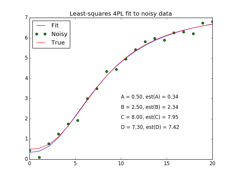
It will be straightforward to modify this code to use, for example, a five parameter logistic or other equation, offering a flexibility rarely available with standard analysis software.
Simulation-based statistics
包括一个bootstrap函数With increasing computational power, it is now feasible to run many, many simulations to estimate parameters instead of, or in addition to, the traditiional parameteric statistial methods. Most of these methods are based on some form of resampling of the data available to estimate the null distribution, with well known examples being the bootstrap and permuation resampling.
Before we do this, we need to understand a little about how to get random numbers. The numpy.random module has random number generators for a variety of common probabiltiy distributions. These numbers are then used to simulate the generation of new random samples. If the samples are chosen in a certain way, the statistics of the randomly drawn samples can provide useful information about the properties of our original data sample. Here are some examples of random number generation in iptyhon.
In [1]: import numpy.random as npr

In [2]: npr.random(5)
Out[2]: array([ 0.88509491,  0.1530188 ,  0.86235945,  0.77324214,  0.27968431])

In [3]: npr.random((3,4))
Out[3]:
array([[ 0.09011934,  0.2435081 ,  0.2463418 ,  0.49527452],
[ 0.54057567,  0.30539368,  0.34848276,  0.64897038],
[ 0.51525096,  0.19594408,  0.86945157,  0.02309191]])

In [4]: npr.normal(5, 1, 4)
Out[4]: array([ 5.39112784,  4.9500269 ,  6.05270335,  5.95333509])

In [5]: npr.randint(1, 7, 10)
Out[5]: array([4, 6, 4, 1, 4, 5, 3, 4, 4, 6])

In [6]: npr.uniform(1, 7, 10)
Out[6]:
array([ 2.04285874,  3.94923612,  5.93212699,  2.39859964,  3.202536  ,
2.30029199,  6.39038325,  4.43109617,  1.93328928,  1.58893167])

In [7]: npr.binomial(n=10, p=0.2, size=(4,4))
Out[7]:
array([[1, 3, 0, 4],
[1, 4, 5, 1],
[5, 2, 1, 0],
[2, 3, 2, 1]])

In [8]: x =  [1,2,3,4,5,6]

In [9]: npr.shuffle(x)

In [10]: x
Out[10]: [4, 3, 6, 2, 1, 5]

In [11]: npr.permutation(10)
Out[11]: array([8, 4, 7, 6, 5, 1, 0, 2, 3, 9])
For example, choosing a new sample with replacement from an existing sample (i.e. we draw one item from the data, record what it is, then replace it in the data and repeat to get a new sample) can be done efficiently in this way:
In [1]: import numpy as np

In [2]: import numpy.random as npr

In [3]: data = np.array(['tom', 'jerry', 'mickey', 'minnie', 'pocahontas'])

In [4]: idx = npr.randint(0, len(data), (4,len(data)))

In [5]: idx
Out[5]:
array([[4, 0, 1, 3, 2],
[4, 1, 0, 1, 4],
[0, 4, 4, 2, 3],
[0, 4, 2, 1, 3]])

In [6]: samples_with_replacement = data[idx]

In [7]: samples_with_replacement
Out[7]:
array([['pocahontas', 'tom', 'jerry', 'minnie', 'mickey'],
['pocahontas', 'jerry', 'tom', 'jerry', 'pocahontas'],
['tom', 'pocahontas', 'pocahontas', 'mickey', 'minnie'],
['tom', 'pocahontas', 'mickey', 'jerry', 'minnie']],
dtype='|S10')
In the next version of numpy (1.7.0), a new function choice is available in numpy.random to do the same thing with a nicer syntax. Version 1.7.0 is only currently available from the git repository as source code that you must compile yourself, but should be available for easy_install/pip installation soon.
In [1]: import numpy.random as npr

In [2]: data = ['tom', 'jerry', 'mickey', 'minnie', 'pocahontas']

# only availlable if you install numpy 1.7.0 from the git repository
In [3]: npr.choice(data, size=(4, len(data)), replace=True)
Out[3]:
array([['tom', 'minnie', 'pocahontas', 'pocahontas', 'pocahontas'],
['minnie', 'tom', 'mickey', 'mickey', 'minnie'],
['minnie', 'pocahontas', 'tom', 'pocahontas', 'mickey'],
['tom', 'mickey', 'jerry', 'jerry', 'mickey']],
dtype='|S10')
Moving on our first simulation example - if we want to plot the 95% confidence interval for the mean of our data samples, we can use the bootstrap to do so. The basic idea is simple - draw many, many samples with replacement from the data available, estimate the mean from each sample, then rank order the means to estimate the 2.5 and 97.5 percentile values for 95% confidence interval. Unlike using normal assumptions to calculate 95% CI, the results generated by the bootstrap are robust even if the underlying data are very far from normal.
import numpy as np
import numpy.random as npr
import matplotlib.pyplot as pylab

def bootstrap(data, num_samples, statistic, alpha):
"""Returns bootstrap estimate of 100.0*(1-alpha) CI for statistic."""
n = len(data)
idx = npr.randint(0, n, (num_samples, n))
samples = data[idx]
stat = np.sort(statistic(samples, 1))
return (stat[int((alpha/2.0)*num_samples)],
stat[int((1-alpha/2.0)*num_samples)])

if __name__ == '__main__':
# data of interest is bimodal and obviously not normal
x = np.concatenate([npr.normal(3, 1, 100), npr.normal(6, 2, 200)])

# find mean 95% CI and 100,000 bootstrap samples
low, high = bootstrap(x, 100000, np.mean, 0.05)

# make plots
pylab.figure(figsize=(8,4))
pylab.subplot(121)
pylab.hist(x, 50, histtype='step')
pylab.title('Historgram of data')
pylab.subplot(122)
pylab.plot([-0.03,0.03], [np.mean(x), np.mean(x)], 'r', linewidth=2)
pylab.scatter(0.1*(npr.random(len(x))-0.5), x)
pylab.plot([0.19,0.21], [low, low], 'r', linewidth=2)
pylab.plot([0.19,0.21], [high, high], 'r', linewidth=2)
pylab.plot([0.2,0.2], [low, high], 'r', linewidth=2)
pylab.xlim([-0.2, 0.3])
pylab.title('Bootstrap 95% CI for mean')
pylab.savefig('boostrap.png')
pylab.show()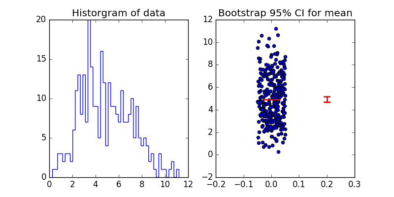
Note that the bootstrap function is a higher order function, and will return the boostrap CI for any valid statistical function, not just the mean. For example, to find the 95% CI for the standard deviation, we only need to change np.mean to np.std in the arguments:
# find standard deviation 95% CI bootstrap samples
low, high =  bootstrap(x, 100000, np.std, 0.05)
The function is also highly optimized, and takes under 2 seconds to calculate the boostrap mean for a data sample of size 300 using 100,000 bootstrap samples on a 4 year old MacBook Pro with 2.4 GHz Intel Core 2 Duo processor.
Permutation-resampling is another form of simulation-based statistical calculation, and is often used to evaluate the p-value for the difference between two groups, under the null hypothesis that the groups are invariant under label permutation.
For example, in a case-control study, it can be used to find the p-value that hypothesis that the mean of the case group is different from that of the control group, and we cannot use the t-test because the distributions are highly skewed.
import numpy as np
import numpy.random as npr
import matplotlib.pyplot as pylab

def permutation_resampling(case, control, num_samples, statistic):
"""Returns p-value that statistic for case is different
from statistc for control."""

observed_diff = abs(statistic(case) - statistic(control))
num_case = len(case)

combined = np.concatenate([case, control])
diffs = []
for i in range(num_samples):
xs = npr.permutation(combined)
diff = np.mean(xs[:num_case]) - np.mean(xs[num_case:])
diffs.append(diff)

pval = (np.sum(diffs > observed_diff) +
np.sum(diffs < -observed_diff))/float(num_samples)
return pval, observed_diff, diffs

if __name__ == '__main__':
# make up some data
case = [94, 38, 23, 197, 99, 16, 141]
control = [52, 10, 40, 104, 51, 27, 146, 30, 46]

# find p-value by permutation resampling
pval, observed_diff, diffs = \
permutation_resampling(case, control, 10000, np.mean)

# make plots
pylab.title('Empirical null distribution for differences in mean')
pylab.hist(diffs, bins=100, histtype='step', normed=True)
pylab.axvline(observed_diff, c='red', label='diff')
pylab.axvline(-observed_diff, c='green', label='-diff')
pylab.text(60, 0.01, 'p = %.3f' % pval, fontsize=16)
pylab.legend()
pylab.savefig('permutation.png')
pylab.show()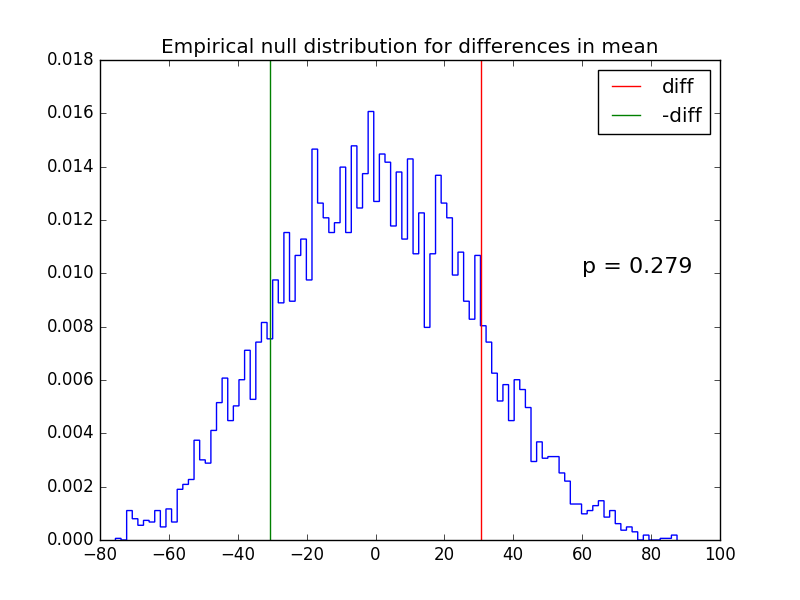

相关文章推荐
- Python动态类型的学习---引用的理解
- Python3写爬虫(四)多线程实现数据爬取
- 垃圾邮件过滤器 python简单实现
- 介绍一款信息管理系统的开源框架---jeecg
- 下载并遍历 names.txt 文件,输出长度最长的回文人名。
- 源码被倒卖,大厂薅羊毛,开源真的只能被予取予求?
- install and upgrade scrapy
- Scrapy的架构介绍
- Centos6 编译安装Python
- bootstrap初试进度条
- 使用Python生成Excel格式的图片
- 让Python文件也可以当bat文件运行
- [Python]推算数独
- Python中zip()函数用法举例
- Python中map()函数浅析
- Bootstrap 3.3.4 发布,Web 前端 UI 框架
- Python将excel导入到mysql中
- 专家解读:开源软件项目是否会被限制出口?