1.1 Built-in Distributions In Matlab

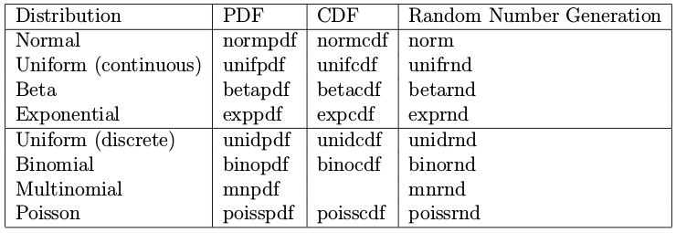
Matlab built-in distributions are all standard distributions, See the summarization below.



Solutions for 1.1.

I‘ve implemented those distributions: illustrate PDF, CDF; Draw random values from them.

(0) Univariate Norm

mu= 102; sigma = 15; % mean and standard deviation
xmin = 70; xmax = 130; % x limitation for pdf and cdf plot
n= 100; % number of points for pdf and cdf plot
k= 10000; % number of random draws for histogram

x= linspace( xmin , xmax , n );%create a set of values ranging from xmin to xmax
p= normpdf( x , mu , sigma ); % calculate the pdf
c= normcdf( x , mu , sigma ); % calculate the cdf

figure( 1 ); clf; % create a new figure and clear the contents
subplot( 1,3,1 );
plot(x,p);
xlabel( 'x' ); ylabel( 'pdf' );
title( 'Probability Density Function' );

subplot( 1,3,2 );
plot( x , c );
xlabel( 'x' ); ylabel( 'cdf' );
title( 'Cumulative Density Function' );

subplot( 1,3,3 );
%draw k random numbers from a N( mu , sigma ) distribution
%here the argument "1" means
y = normrnd( mu , sigma , k , 1 );
hist( y , 20 );%20 bars
xlabel( 'x' ); ylabel( 'frequency' );
title( 'Histogram of random values' );

pause;

(1) Beta

alpha= 2; beta = 3; %parameters
xmin = 0; xmax = 1; % x limitation for pdf and cdf plot
n= 100; % number of points for pdf and cdf plot
k= 10000; % number of random draws for histogram

x= linspace( xmin , xmax , n );%create a set of values ranging from xmin to xmax
p= betapdf( x , alpha , beta ); % calculate the pdf
c= betacdf( x , alpha , beta); % calculate the cdf

figure( 1 ); clf; % create a new figure and clear the contents
subplot( 1,3,1 );
plot(x,p);
xlabel( 'x' ); ylabel( 'pdf' );
title( 'Probability Density Function' );

subplot( 1,3,2 );
plot( x , c );
xlabel( 'x' ); ylabel( 'cdf' );
title( 'Cumulative Density Function' );

subplot( 1,3,3 );
%draw k random numbers from a N( mu , sigma ) distribution
%here the argument "1" means
y = betarnd( alpha , beta , k , 1 );
hist( y , 20 );%20 bars
xlabel( 'x' ); ylabel( 'frequency' );
title( 'Histogram of random values' );

pause;

(1) Exponential

gamma=2; % parameters
xmin = 1; xmax = 7; % x limitation for pdf and cdf plot
n= 100; % number of points for pdf and cdf plot
k= 10000; % number of random draws for histogram

x= linspace( xmin , xmax , n );%create a set of values ranging from xmin to xmax
p= exppdf( x , gamma ); % calculate the pdf
c= expcdf( x , gamma); % calculate the cdf

figure( 1 ); clf; % create a new figure and clear the contents
subplot( 1,3,1 );
plot(x,p);
xlabel( 'x' ); ylabel( 'pdf' );
title( 'Probability Density Function' );

subplot( 1,3,2 );
plot( x , c );
xlabel( 'x' ); ylabel( 'cdf' );
title( 'Cumulative Density Function' );

subplot( 1,3,3 );
%draw k random numbers from a N( mu , sigma ) distribution
%here the argument "1" means
y = exprnd( gamma, k , 1 );
hist( y , 20 );%20 bars
xlabel( 'x' ); ylabel( 'frequency' );
title( 'Histogram of random values' );

pause;

(2) Binomial

N= 10; theta = 0.7; % parameters
xmin = 0; xmax = 10; % x limitation for pdf and cdf plot
n= 100; % number of points for pdf and cdf plot
k= 10000; % number of random draws for histogram

x= linspace( xmin , xmax , n );%create a set of values ranging from xmin to xmax
p= binopdf( x , N , theta ); % calculate the pdf
c= binocdf( x , N , theta); % calculate the cdf

figure( 1 ); clf; % create a new figure and clear the contents
subplot( 1,3,1 );
plot(x,p);
xlabel( 'x' ); ylabel( 'pdf' );
title( 'Probability Density Function' );

subplot( 1,3,2 );
plot( x , c );
xlabel( 'x' ); ylabel( 'cdf' );
title( 'Cumulative Density Function' );

subplot( 1,3,3 );
%draw k random numbers from a N( mu , sigma ) distribution
%here the argument "1" means
y = binornd( N , theta , k , 1 );
hist( y , 20 );%20 bars
xlabel( 'x' ); ylabel( 'frequency' );
title( 'Histogram of random values' );

pause;

(4) Uniform

a= 5; b = 10; %parameters
xmin = 4; xmax = 11; % x limitation for pdf and cdf plot
n= 100; % number of points for pdf and cdf plot
k= 10000; % number of random draws for histogram

x= linspace( xmin , xmax , n );%create a set of values ranging from xmin to xmax
p= unifpdf( x , a , b ); % calculate the pdf
c= unifcdf( x , a , b ); % calculate the cdf

figure( 1 ); clf; % create a new figure and clear the contents
subplot( 1,3,1 );
plot(x,p);
xlabel( 'x' ); ylabel( 'pdf' );
title( 'Probability Density Function' );

subplot( 1,3,2 );
plot( x , c );
xlabel( 'x' ); ylabel( 'cdf' );
title( 'Cumulative Density Function' );

subplot( 1,3,3 );
%draw k random numbers from a N( mu , sigma ) distribution
%here the argument "1" means
y = unifrnd( a , b , k , 1 );
hist( y , 20 );%20 bars
xlabel( 'x' ); ylabel( 'frequency' );
title( 'Histogram of random values' );

pause;

(4) Generate identical replica

a= 0; b = 1;
n= 10;
seed=1;
rand('state',seed); randn('state',seed);
unifrnd(a,b,n,1)
%'state'是对随机发生器的状态进行初始化，并且定义该状态初始值。比如你过一段时间还要使用这个随机数的时候，还能保持当前的随机取值。
%比如
%randn('state',2013)
%a = randn(1)
%b = randn(1) 会发现与上一个随机值不一样
%如果再定义一次
%randn('state',2013)
%c = randn(1) 会发现与a的值一样
rand('state',seed); randn('state',seed);
unifrnd(a,b,n,1)

(5) IQ Probalility

normcdf(130,100,15)-normcdf(110,100,15)