UFLDL教程答案(8):Exercise:Convolution and Pooling
2015-12-27 11:36
537 查看
教程地址:http://deeplearning.stanford.edu/wiki/index.php/UFLDL%E6%95%99%E7%A8%8B
练习地址:http://deeplearning.stanford.edu/wiki/index.php/Exercise:Convolution_and_Pooling
卷积神经网络结构可以看教程或者
/article/1919457.html
(1)局部连接与权值共享:
之前使用的mnist数据集28*28小图片使用全连接计算不会太慢,但如果是自然图片98*98,你需要设计近10 的 4 次方(100*100)个输入单元,假设你要学习 100 个特征,那么就有 10 的 6 次方个参数需要去学习。不管是前向传播还是反向传播都会很慢。
所以:每个隐含单元仅仅只能连接输入单元的一部分。例如,每个隐含单元仅仅连接输入图像的一小片相邻区域。这就是局部连接。
局部连接与权值共享不单单是为了减少计算量,这种方式是受人脑视觉神经系统启发设计的。设计原因有俩点:
1.自然图像中局部信息是高度相关的,形成局部motifs(这个词不知道该翻译成什么好,有点只可意会不可言传的感觉);
2.图像的局部统计特性对位置具有不变性,也就是说如果motifs出现在图像的某个地方,它也可以出现在任何其他地方。所以权值共享可以在图片的各个地方挖掘出相同的模式(一个feature map就挖掘一种模式)。

绿色为原图5*5,黄色为某个卷积核 3*3,红色3*3就是得到的一个feature map,为原图与此卷积核卷积的结果(也可以说原图被提取的特征)
注意有:feature map的3*3=(5-3+1)*(5-3+1),等式右边5为绿色长宽,3为黄色长宽
(2)池化:
虽然前面已经减少了很多参数,但是计算量还是很大,并且容易出现过拟合 (over-fitting),所以需要池化。
池化一般是最大值池化和平均值池化。
池化是平移不变性 (translation invariant)的关键。这就意味着即使图像经历了一个小的平移或者形变之后,依然会产生相同的 (池化的) 特征。
(3)网络结构:
输入层:为 64*64的图片,每张图RGB3个通道,64*64的大小,一共2000张训练样本。
卷积层:卷积核为 8*8,由前一个练习训练得到 W(400*192),b(400*1),其中192=8*8*3,代表8*8小图像块3通道的所有元素的权重,400表示400个不同的卷积核,即最终生成400个不同的feature map(每个大小为57*57,57=64-8+1)。
池化层:400个57*57的feature map被池化成400个3*3。
输出层:softmax层输入为400*3*3,输出4类(airplane, car, cat, dog)。
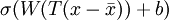
, whereT
is the whitening matrix and

is the mean patch. Expanding this, you obtain
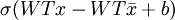
,
which suggests that you should convolve the images withWT rather thanW as earlier, and you should add

,
rather than justb to convolvedFeatures, before finally applying the sigmoid function.
(2)im = squeeze(images(:, :, channel, imageNum));
这句可以看出squeeze函数就是去除维数为1的维度,如这句中channel,imageNum这两个维度维数都为1,被去除。
(3)conv2(im,feature,'valid');
conv2函数第3个参数shape=valid时,卷积时不考虑边界补零,即使输出矩阵维度为(imageDim - patchDim + 1, imageDim - patchDim + 1)
cnnConvolve.m
测试结果:Congratulations! Your pooling code passed the test.
(2)B = permute(A,order)
按照向量order指定的顺序重排A的各维。B中元素和A中元素完全相同。但由于经过重新排列,在A、B访问同一个元素使用的下标就不一样了。order中的元素必须各不相同。
--> A =
randn(13,5,7,2);
--> size(A)
ans = 13 5 7 2
--> B = permute(A,[3,4,2,1]);
--> size(B)
ans = 7 2 5 13
即各维度调整了顺序,读数据时下标改变了。
(3)注意把需要的文件拷贝过来,程序跑完挺废时间的,所以保存好中间变量:
save('cnnPooledFeatures.mat', 'pooledFeaturesTrain', 'pooledFeaturesTest');
(4)结果:

练习地址:http://deeplearning.stanford.edu/wiki/index.php/Exercise:Convolution_and_Pooling
1.要点简述
卷积神经网络4个核心点:
局部连接,权重共享,池化,多层。卷积神经网络结构可以看教程或者
/article/1919457.html
(1)局部连接与权值共享:
之前使用的mnist数据集28*28小图片使用全连接计算不会太慢,但如果是自然图片98*98,你需要设计近10 的 4 次方(100*100)个输入单元,假设你要学习 100 个特征,那么就有 10 的 6 次方个参数需要去学习。不管是前向传播还是反向传播都会很慢。
所以:每个隐含单元仅仅只能连接输入单元的一部分。例如,每个隐含单元仅仅连接输入图像的一小片相邻区域。这就是局部连接。
局部连接与权值共享不单单是为了减少计算量,这种方式是受人脑视觉神经系统启发设计的。设计原因有俩点:
1.自然图像中局部信息是高度相关的,形成局部motifs(这个词不知道该翻译成什么好,有点只可意会不可言传的感觉);
2.图像的局部统计特性对位置具有不变性,也就是说如果motifs出现在图像的某个地方,它也可以出现在任何其他地方。所以权值共享可以在图片的各个地方挖掘出相同的模式(一个feature map就挖掘一种模式)。
绿色为原图5*5,黄色为某个卷积核 3*3,红色3*3就是得到的一个feature map,为原图与此卷积核卷积的结果(也可以说原图被提取的特征)
注意有:feature map的3*3=(5-3+1)*(5-3+1),等式右边5为绿色长宽,3为黄色长宽
(2)池化:
虽然前面已经减少了很多参数,但是计算量还是很大,并且容易出现过拟合 (over-fitting),所以需要池化。
池化一般是最大值池化和平均值池化。
池化是平移不变性 (translation invariant)的关键。这就意味着即使图像经历了一个小的平移或者形变之后,依然会产生相同的 (池化的) 特征。
(3)网络结构:
输入层:为 64*64的图片,每张图RGB3个通道,64*64的大小,一共2000张训练样本。
卷积层:卷积核为 8*8,由前一个练习训练得到 W(400*192),b(400*1),其中192=8*8*3,代表8*8小图像块3通道的所有元素的权重,400表示400个不同的卷积核,即最终生成400个不同的feature map(每个大小为57*57,57=64-8+1)。
池化层:400个57*57的feature map被池化成400个3*3。
输出层:softmax层输入为400*3*3,输出4类(airplane, car, cat, dog)。
2.进入正题
Step 2a: Implement convolution
(1)Taking the preprocessing steps into account, the feature activations that you should compute is, whereT
is the whitening matrix and
is the mean patch. Expanding this, you obtain
,
which suggests that you should convolve the images withWT rather thanW as earlier, and you should add
,
rather than justb to convolvedFeatures, before finally applying the sigmoid function.
(2)im = squeeze(images(:, :, channel, imageNum));
这句可以看出squeeze函数就是去除维数为1的维度,如这句中channel,imageNum这两个维度维数都为1,被去除。
(3)conv2(im,feature,'valid');
conv2函数第3个参数shape=valid时,卷积时不考虑边界补零,即使输出矩阵维度为(imageDim - patchDim + 1, imageDim - patchDim + 1)
cnnConvolve.m
function convolvedFeatures = cnnConvolve(patchDim, numFeatures, images, W, b, ZCAWhite, meanPatch)
%cnnConvolve Returns the convolution of the features given by W and b with
%the given images
%
% Parameters:
%  patchDim - patch (feature) dimension
%  numFeatures - number of features
%  images - large images to convolve with, matrix in the form
%           images(r, c, channel, image number)
%  W, b - W, b for features from the sparse autoencoder
%  ZCAWhite, meanPatch - ZCAWhitening and meanPatch matrices used for
%                        preprocessing
%
% Returns:
%  convolvedFeatures - matrix of convolved features in the form
%                      convolvedFeatures(featureNum, imageNum, imageRow, imageCol)

numImages = size(images, 4);
imageDim = size(images, 1);
imageChannels = size(images, 3);

convolvedFeatures = zeros(numFeatures, numImages, imageDim - patchDim + 1, imageDim - patchDim + 1);

% Instructions:
%   Convolve every feature with every large image here to produce the
%   numFeatures x numImages x (imageDim - patchDim + 1) x (imageDim - patchDim + 1)
%   matrix convolvedFeatures, such that
%   convolvedFeatures(featureNum, imageNum, imageRow, imageCol) is the
%   value of the convolved featureNum feature for the imageNum image over
%   the region (imageRow, imageCol) to (imageRow + patchDim - 1, imageCol + patchDim - 1)
%
% Expected running times:
%   Convolving with 100 images should take less than 3 minutes
%   Convolving with 5000 images should take around an hour
%   (So to save time when testing, you should convolve with less images, as
%   described earlier)

% -------------------- YOUR CODE HERE --------------------
% Precompute the matrices that will be used during the convolution. Recall
% that you need to take into account the whitening and mean subtraction
% steps
WT=W*ZCAWhite;   %(400*192)*(192*192)   400是hiddenSize代表400种不同的feature map
B=b-WT*meanPatch;%(400*1) 这两步是根据教程step2a末尾的建议
% --------------------------------------------------------
convolvedFeatures = zeros(numFeatures, numImages, imageDim - patchDim + 1, imageDim - patchDim + 1);
for imageNum = 1:numImages
for featureNum = 1:numFeatures

% convolution of image with feature matrix for each channel
convolvedImage = zeros(imageDim - patchDim + 1, imageDim - patchDim + 1);
for channel = 1:3

% Obtain the feature (patchDim x patchDim) needed during the convolution
% ---- YOUR CODE HERE ----
%feature = zeros(8,8); % You should replace this
temp=patchDim*patchDim;
feature=reshape(WT(featureNum,1+(channel-1)*temp:channel*temp),patchDim,patchDim);
% ------------------------

% Flip the feature matrix because of the definition of convolution, as explained later
feature = flipud(fliplr(squeeze(feature)));

% Obtain the image
im = squeeze(images(:, :, channel, imageNum));%squeeze会消除只有1维的维度

% Convolve "feature" with "im", adding the result to convolvedImage
% 3通道都卷积后需要求和得到convolvedImage
% be sure to do a 'valid' convolution
% ---- YOUR CODE HERE ----
convolvedChannel=conv2(im,feature,'valid');%shape=valid时,卷积时不考虑边界补零
convolvedImage=convolvedImage+convolvedChannel;
% ------------------------

end

% Subtract the bias unit (correcting for the mean subtraction as well)
% Then, apply the sigmoid function to get the hidden activation
% ---- YOUR CODE HERE ----
convolvedImage=sigmoid(convolvedImage+B(featureNum));  %根据教程step2a末尾的建议

% ------------------------

% The convolved feature is the sum of the convolved values for all channels
convolvedFeatures(featureNum, imageNum, :, :) = convolvedImage;
end
end

end

function sigm = sigmoid(x)

sigm = 1 ./ (1 + exp(-x));
end
Step 2b: Check your convolution
运行自带的测试代码,显示:Congratulations! Your convolution code passed the test. 卷积代码无误!Step 2c: Pooling
池化代码较为容易,使用卷积中类似for循环即可。%采用和cnnConvolve.m中的循环顺序 pooledDim=floor(convolvedDim/poolDim); for imageNum = 1:numImages for featureNum = 1:numFeatures for poolRow = 1:pooledDim for poolCol = 1:pooledDim poolMatrix = convolvedFeatures(featureNum, imageNum, (poolRow-1)*poolDim+1:poolRow*poolDim, (poolCol-1)*poolDim+1:poolCol*poolDim); pooledFeatures(featureNum, imageNum, poolRow, poolCol) = mean(poolMatrix(:)); end end end end
测试结果:Congratulations! Your pooling code passed the test.
结果:
(1)后面的代码NG已经给出,设置了stepSize = 50; 是为了避免内存溢出,分400/50=8次来计算,每次算50种feature map。如果电脑运行起来卡,把这个值改小些,改成10,20之类的。(2)B = permute(A,order)
按照向量order指定的顺序重排A的各维。B中元素和A中元素完全相同。但由于经过重新排列,在A、B访问同一个元素使用的下标就不一样了。order中的元素必须各不相同。
--> A =
randn(13,5,7,2);
--> size(A)
ans = 13 5 7 2
--> B = permute(A,[3,4,2,1]);
--> size(B)
ans = 7 2 5 13
即各维度调整了顺序,读数据时下标改变了。
(3)注意把需要的文件拷贝过来,程序跑完挺废时间的,所以保存好中间变量:
save('cnnPooledFeatures.mat', 'pooledFeaturesTrain', 'pooledFeaturesTest');
(4)结果:

相关文章推荐
- 如何 copy 文件到 mac 上的 ntfs 格式移动硬盘中
- nyoj801 Haffman编码(优先队列实现)
- ArrayList及HashMap的扩容规则
- C++ Stack Implementation Discussion
- 摄像机内外参数
- [leetcode] 26. Remove Duplicates from Sorted Array 解题报告
- 常用算法回顾——二分查找算法
- 细说五层网站架构
- MyBatis经典入门实例
- Java中有关Null的9件事
- memcached之java客户端:spymemcached与spring整合
- 将函数名(地址)作为参数传递
- 自然语言处理
- CentOS 7部署OpenStack(1)-―准备基础环境
- List#toArray小技巧
- Android 图形 II-OpenGL ES
- 华为oj:判断两个IP是否属于同一个子网
- 通知栏通知:Notification的实现
- atitit.团队建设--要不要招技术储备人才的问题
- 课程总结报告