尺度不变特征转换SIFT
2015-12-16 21:21
190 查看
The Scale-Invariant Feature Transform (SIFT) bundles a feature detector and a feature descriptor. The detector extracts from an image a number
of frames (attributed regions) in a way which is consistent with (some) variations of the illumination, viewpoint and other viewing conditions. The descriptor associates to the regions a signature which identifies their appearance compactly and robustly. For
a more in-depth description of the algorithm, see our API reference for SIFT.
command (there is a similar command line utility). Open MATLAB and load a test image
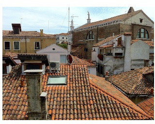
Input image.
The
requires a single precision gray scale image. It also expects the range to be normalized in the [0,255] interval (while this is not strictly required, the default values of some internal thresholds are tuned for this case). The image
converted in the appropriate format by
We compute the SIFT frames (keypoints) and descriptors by
The matrix
scale
We visualize a random selection of 50 features by:
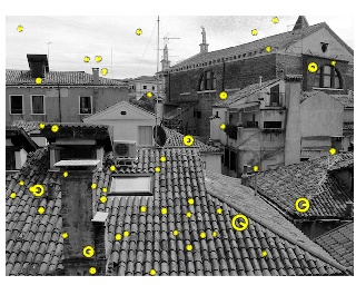
Some of the detected SIFT frames.
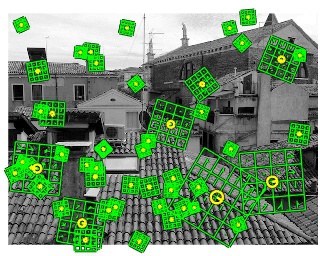
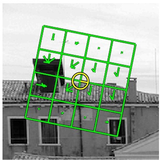
We can also overlay the descriptors by
A test image for the peak threshold parameter.
a basic matching algorithm. Let
images of the same object or scene. We extract and match the descriptors by:
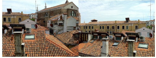
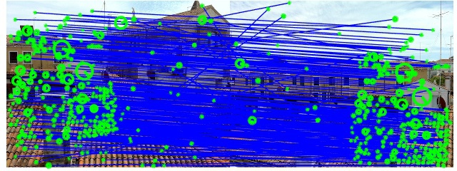
Top: A pair of images of the same scene. Bottom: Matching of SIFT descriptors with
For each descriptor in
the closest descriptor in
descriptor is stored in each column of
Matches also can be filtered for uniqueness by passing a third parameter to
specifies a threshold. Here, the uniqueness of a pair is measured as the ratio of the distance between the best matching keypoint and the distance to the second best one (see
further details).
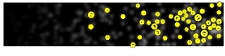
The peak threshold filters peaks of the DoG scale space that are too small (in absolute value). For instance, consider a test image of 2D Gaussian blobs:
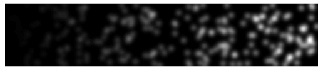
A test image for the peak threshold parameter.
We run the detector with peak threshold
obtaining fewer features as
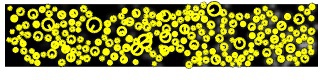
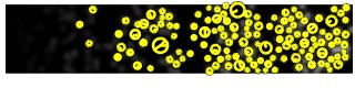
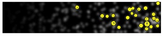
Detected frames for increasing peak threshold.
From top:
The edge threshold eliminates peaks of the DoG scale space whose curvature is too small (such peaks yield badly localized frames). For instance, consider the test image
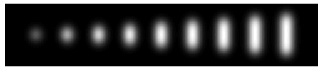
A test image for the edge threshold parameter.
We run the detector with edge threshold
obtaining more features as
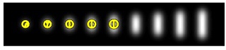
Detected frames for increasing edge threshold.
From top:
the command line utility) can bypass the detector and compute the descriptor on custom frames using the
For instance, we can compute the descriptor of a SIFT frame centered at position
orientation
Custom frame at with fixed orientation.
Multiple frames
instructs the program to use the custom position and scale but to compute the keypoint orientations, as in
Custom frame with computed orientations.
Notice that, depending on the local appearance, a keypoint may have multiple orientations. Moreover, a keypoint computed on a constant image region (such as a one pixel region) has no orientations!
(0,0). Lowe's original implementation uses a different reference system, illustrated next:
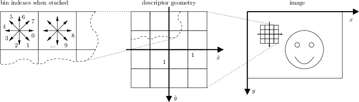
Our conventions (top) compared to Lowe's (bottom).
Our implementation uses the standard image reference system, with the
descriptor use the same reference system (i.e. a small positive rotation of the
Recall that each descriptor element is a bin indexed by
the fastest varying index and
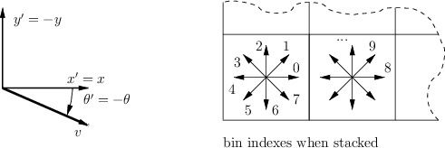
By comparison, D. Lowe's implementation (see bottom half of the figure) uses a slightly different convention: Frame centers are expressed relatively to the standard image reference system, but the frame orientation and the descriptor assume that
the y axis points upward. Consequently, to map from our to D. Lowe's convention, frames orientations need to be negated and the descriptor elements must be re-arranged.
are stored in a slightly different format, see
The following figure compares SIFT keypoints computed by the VLFeat (blue) and UBC (red) implementations.
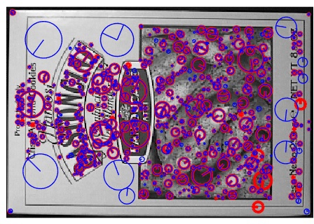
VLFeat keypoints (blue) superimposed to D. Lowe's keypoints (red). Most keypoints match nearly exactly.
The large majority of keypoints correspond nearly exactly. The following figure shows the percentage of keypoints computed by the two implementations whose center matches with a precision of at least 0.01 pixels and 0.05 pixels respectively.
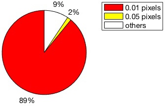
Percentage of keypoints obtained from the VLFeat and UBC implementations that match up to 0.01 pixels and 0.05 pixels.
Descriptors are also very similar. The following figure shows the percentage of descriptors computed by the two implementations whose distance is less than 5%, 10% and 20% of the average descriptor distance.
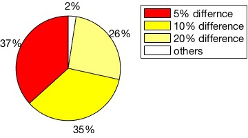
Percentage of descriptors obtained from the VLFeat and UBC implementations whose distance is within 10% and 20% of the average descriptor distance.
from: http://www.vlfeat.org/overview/sift.html
of frames (attributed regions) in a way which is consistent with (some) variations of the illumination, viewpoint and other viewing conditions. The descriptor associates to the regions a signature which identifies their appearance compactly and robustly. For
a more in-depth description of the algorithm, see our API reference for SIFT.
Extracting frames and descriptors
Both the detector and descriptor are accessible by thevl_siftMATLAB
command (there is a similar command line utility). Open MATLAB and load a test image
I = vl_impattern('roofs1') ;
image(I) ;
Input image.
The
vl_siftcommand
requires a single precision gray scale image. It also expects the range to be normalized in the [0,255] interval (while this is not strictly required, the default values of some internal thresholds are tuned for this case). The image
Iis
converted in the appropriate format by
I = single(rgb2gray(I)) ;
We compute the SIFT frames (keypoints) and descriptors by
[f,d] = vl_sift(I) ;
The matrix
fhas a column for each frame. A frame is a disk of center
f(1:2),
scale
f(3)and orientation
f(4).
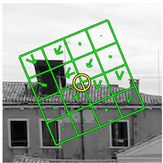
We visualize a random selection of 50 features by:
perm = randperm(size(f,2)) ;
sel = perm(1:50) ;
h1 = vl_plotframe(f(:,sel)) ;
h2 = vl_plotframe(f(:,sel)) ;
set(h1,'color','k','linewidth',3) ;
set(h2,'color','y','linewidth',2) ;
Some of the detected SIFT frames.
We can also overlay the descriptors by
h3 = vl_plotsiftdescriptor(d(:,sel),f(:,sel)) ;
set(h3,'color','g') ;
A test image for the peak threshold parameter.
Basic matching
SIFT descriptors are often used find similar regions in two images.vl_ubcmatchimplements
a basic matching algorithm. Let
Iaand
Ibbe
images of the same object or scene. We extract and match the descriptors by:
[fa, da] = vl_sift(Ia) ;
[fb, db] = vl_sift(Ib) ;
[matches, scores] = vl_ubcmatch(da, db) ;
Top: A pair of images of the same scene. Bottom: Matching of SIFT descriptors with
vl_ubcmatch.
For each descriptor in
da,
vl_ubcmatchfinds
the closest descriptor in
db(as measured by the L2 norm of the difference between them). The index of the original match and the closest
descriptor is stored in each column of
matchesand the distance between the pair is stored in
scores.
Matches also can be filtered for uniqueness by passing a third parameter to
vl_ubcmatchwhich
specifies a threshold. Here, the uniqueness of a pair is measured as the ratio of the distance between the best matching keypoint and the distance to the second best one (see
vl_ubcmatchfor
further details).
Detector parameters
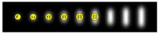
The SIFT detector is controlled mainly by two parameters: the peak threshold and the (non) edge threshold.The peak threshold filters peaks of the DoG scale space that are too small (in absolute value). For instance, consider a test image of 2D Gaussian blobs:
I = double(rand(100,500) <= .005) ;
I = (ones(100,1) * linspace(0,1,500)) .* I ;
I(:,1) = 0 ; I(:,end) = 0 ;
I(1,:) = 0 ; I(end,:) = 0 ;
I = 2*pi*4^2 * vl_imsmooth(I,4) ;
I = single(255 * I) ;
A test image for the peak threshold parameter.
We run the detector with peak threshold
peak_threshby
f = vl_sift(I, 'PeakThresh', peak_thresh) ;
obtaining fewer features as
peak_threshis increased.
Detected frames for increasing peak threshold.
From top:
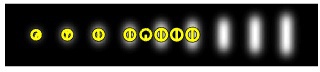
peak_thresh = {0, 10, 20, 30}.The edge threshold eliminates peaks of the DoG scale space whose curvature is too small (such peaks yield badly localized frames). For instance, consider the test image
I = zeros(100,500) ;
for i=[10 20 30 40 50 60 70 80 90]
I(50-round(i/3):50+round(i/3),i*5) = 1 ;
end
I = 2*pi*8^2 * vl_imsmooth(I,8) ;
I = single(255 * I) ;
A test image for the edge threshold parameter.
We run the detector with edge threshold
edge_threshby
f = vl_sift(I, 'edgethresh', edge_thresh) ;
obtaining more features as
edge_threshis increased:
Detected frames for increasing edge threshold.
From top:
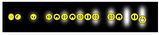
edge_thresh = {3.5, 5, 7.5, 10}Custom frames
The MATLAB commandvl_sift(and
the command line utility) can bypass the detector and compute the descriptor on custom frames using the
Framesoption.
For instance, we can compute the descriptor of a SIFT frame centered at position
(100,100), of scale
10and
orientation
-pi/8by
fc = [100;100;10;-pi/8] ;
[f,d] = vl_sift(I,'frames',fc) ;
Custom frame at with fixed orientation.
Multiple frames
fcmay be specified as well. In this case they are re-ordered by increasing scale. The
Orientationsoption
instructs the program to use the custom position and scale but to compute the keypoint orientations, as in
fc = [100;100;10;0] ;
[f,d] = vl_sift(I,'frames',fc,'orientations') ;
Custom frame with computed orientations.
Notice that, depending on the local appearance, a keypoint may have multiple orientations. Moreover, a keypoint computed on a constant image region (such as a one pixel region) has no orientations!
Conventions
In our implementation SIFT frames are expressed in the standard image reference. The only difference between the command line and MATLAB drivers is that the latter assumes that the image origin (top-left corner) has coordinate (1,1) as opposed to(0,0). Lowe's original implementation uses a different reference system, illustrated next:
Our conventions (top) compared to Lowe's (bottom).
Our implementation uses the standard image reference system, with the
yaxis pointing downward. The frame orientation
θand
descriptor use the same reference system (i.e. a small positive rotation of the
xmoves it towards the
yaxis).
Recall that each descriptor element is a bin indexed by
(θ,x,y); the histogram is vectorized in such a way that
θis
the fastest varying index and
ythe slowest.
By comparison, D. Lowe's implementation (see bottom half of the figure) uses a slightly different convention: Frame centers are expressed relatively to the standard image reference system, but the frame orientation and the descriptor assume that
the y axis points upward. Consequently, to map from our to D. Lowe's convention, frames orientations need to be negated and the descriptor elements must be re-arranged.
Comparison with D. Lowe's SIFT
VLFeat SIFT implementation is largely compatible with UBC (D. Lowe's) implementation (note however that the keypointsare stored in a slightly different format, see
vl_ubcread).
The following figure compares SIFT keypoints computed by the VLFeat (blue) and UBC (red) implementations.
VLFeat keypoints (blue) superimposed to D. Lowe's keypoints (red). Most keypoints match nearly exactly.
The large majority of keypoints correspond nearly exactly. The following figure shows the percentage of keypoints computed by the two implementations whose center matches with a precision of at least 0.01 pixels and 0.05 pixels respectively.
Percentage of keypoints obtained from the VLFeat and UBC implementations that match up to 0.01 pixels and 0.05 pixels.
Descriptors are also very similar. The following figure shows the percentage of descriptors computed by the two implementations whose distance is less than 5%, 10% and 20% of the average descriptor distance.
Percentage of descriptors obtained from the VLFeat and UBC implementations whose distance is within 10% and 20% of the average descriptor distance.
from: http://www.vlfeat.org/overview/sift.html

相关文章推荐
- 智能防火墙的技术特征
- C#图像处理之霓虹效果实现方法
- C#图像亮度调整的方法
- C#实现图像锐化的方法
- C#图像透明度调整的方法
- C#数字图象处理之图像灰度化方法
- C#图像处理之头发检测的方法
- C#图像处理之图像目标质心检测的方法
- C#实现图像反色的方法
- 从jsp发送动态图像
- C#数字图像处理之图像缩放的方法
- C++将CBitmap类中的图像保存到文件的方法
- C#图像重新着色的方法
- 使用CamanJS在Web页面上处理图像的技巧
- PHP图像处理类库MagickWand用法实例分析
- php图像处理类实例
- php对图像的各种处理函数代码小结
- C#控制图像旋转和翻转的方法
- C#实现在图像中绘制文字图形的方法
- C#数字图像处理之图像二值化(彩色变黑白)的方法