数据分析之美：如何进行回归分析

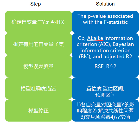
1. 确定自变量与Y是否相关

证明：自变量X1，X2，....XP中至少存在一个自变量与因变量Y相关
For any given value of n（观测数据的数目） and p（自变量X的数目）, any statistical software  package can be used to compute the p-value associated with the F-statistic using this distribution. Based on this p-value, we can determine whether or not to reject H0. （用软件计算出的与F-statistic
相关的p-value来验证假设，the p-value associated with the F-statistic）

例子：

Is there a relationship between advertising sales（销售额） and budget（广告预算：TV, radio, and newspaper）?
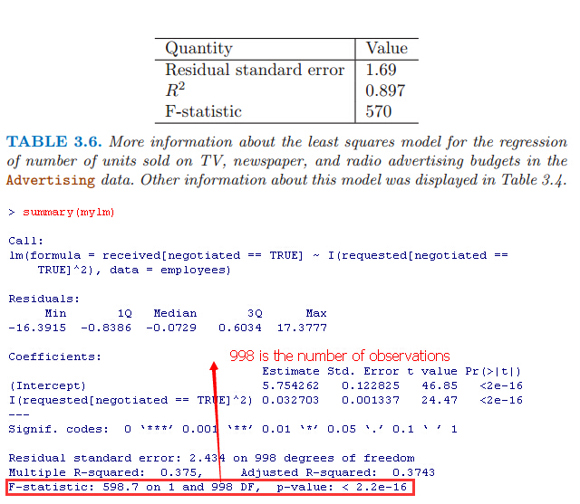
the p-value corresponding to the F-statistic in Table 3.6 is very low, indicating clear evidence of a relationship between advertising and sales.



背景知识回顾：

t-statistic T统计量（t检验）与F-statistic

t-statistic T统计量=（回归系数β的估计值-0）/β的标准误 ，which measures the number of standard deviations thatβis away from 0。用来对计量经济学模型中关于参数的单个假设进行检验的一种统计量。 
我们一般用t统计量来检验回归系数是否为0做检验。例如：线性回归Y=β0+β1X，为了验证X与Y是否相关， 
假设H0：X与Y无关,即β1=0
假设H1：X与Y相关,即β1不等于0
计算t-statistic， 如果t-statistic is far away from zero,则x和y相关。一般用p-values来检验X和Y是否相关。

1）p-values（Probability，Pr）
1 定义
pvalue的定义：在原假设正确的情况下，出现当前情况或者更加极端情况的概率。
p值是用来衡量统计显著性的常用指标。
P值( P-Value，Probability，Pr）即概率，反映某一事件发生的可能性大小。统计学根据显著性检验方法所得到的P 值，一般以P < 0.05 为显著， P <0.01 为非常显著，其含义是样本间的差异由抽样误差所致的概率小于0.05 或0.01。实际上，P 值不能赋予数据任何重要性，只能说明某事件发生的机率。

假设检验是推断统计中的一项重要内容。在假设检验中常见到P 值( P-Value，Probability，Pr)，P 值是进行检验决策的另一个依据。
大的pvalue说明还没有足够的证据拒绝原假设。

2 为何有p-value
P值方法的思路是先进行一项实验，然后观察实验结果是否符合随机结果的特征。研究人员首先提出一个他们想要推翻的“零假设”（null hypothesis），比如，两组数据没有相关性或两组数据没有显著差别。接下来，他们会故意唱反调，假设零假设是成立的，然后计算实际观察结果与零假设相吻合的概率。这个概率就是P值。费希尔说，P值越小，研究人员成功证明这个零假设不成立的可能性就越大。

其实理解起来很简单，基本原理只有两个：
1）一个命题只能证伪，不能证明为真
2）小概率事件不可能发生

证明逻辑就是：我要证明命题为真->证明该命题的否命题为假->在否命题的假设下，观察到小概率事件发生了->搞定。

3 demo
投飞镖，假设一个飞镖有10，9,8,7,6,5,4,3,2,1总共十个环（10是中心），定义合格投手为其真实水平能投到10~3环，而不管他临场表现如何。假设10~3环占靶子面积的95%。
H0：A是一个合格投手
H1：A不是合格投手

结合这个例子来看：证明A是合格的投手-》证明“A不是合格投手”的命题为假-》观察到一个事件（比如A连续10次投中10环），而这个事件在“A不是合格投手”的假设下，概率为p，小于0.05->小概率事件发生，否命题被推翻。

可以看到p越小-》这个事件越是小概率事件-》否命题越可能被推翻-》原命题越可信

2）F-statistic
t检验是单个系数显著性的检验，检验一个变量X与Y是否相关，如电视上广告投入是否有利于销售额。T检验的原假设为某一解释变量的系数为0 。
F检验是是所有的自变量在一起对因变量的影响，当处理3个及其以上的时候（变量X1，X2，X3...等）用的是F检验。F检验的原假设为所有回归系数为0。
即F检验用于证明变量X1，X2，X3...中至少有一个变量和Y相关

F检验的原假设是H0：所有回归参数都等于0，所以F检验通过的话说明模型总体存在，F检验不通过，其他的检验就别做了，因为模型所有参数不显著异于0，相当于模型不存在（即没有任何一个变量X1，X2，X3... have no relationship with Y）。

2.确定有用的自变量子集

Do all the predictors help to explain Y , or is only a subset of the  predictors useful? （确定对Y有用的自变量）

The first step in a multiple regression analysis is to compute the F-statistic and to examine the associated pvalue. If we conclude on the basis of that p-value that at least one of the predictors is related to the response, then it is natural to wonder which are the
guilty ones!

The task of determining which predictors are associated with the response, in order to fit a single model involving only those predictors, is referred to as variable selection.

There are three classical approaches for this task:Forward selection.Forward selection.Forward selection.
1）Forward selection. 
We begin with the null model—a model that conforward  selection null model tains an intercept but no predictors. We then fit p simple linear regressions 
and add to the null model the variable that results in the  lowest RSS. We then add to that model the variable that results in the lowest RSS for the new two-variable model. This approach is  continued until some stopping rule is satisfied.

2)Backward selection. 
We start with all variables in the model, and  backward remove the variable with the largest p-value—that is, the variable selection that is the least statistically significant. The new (p − 1)-variable model is fit, and the variable with the largest p-value
is removed. This procedure continues until a stopping rule is reached. For instance, we may stop when all remaining variables have a p-value below some threshold.

3)Mixed selection. 
This is a combination of forward and backward semixed  lection. We start with no variables in the model, and as with forward selection , we add the variable that provides the best fit. We continue to add variables one-by-one. Of course, as we noted with
the Advertising example, the p-values for variables can become larger as new predictors are added to the model. Hence, if at any point the p-value for one of the variables in the model rises above a certain threshold, then we remove that variable from the
model. We continue to perform these forward and backward steps until all variables in the model have a sufficiently low p-value, and all variables outside the model would have a large p-value if added to the model.

Compare:
Backward selection requires that the number of samples n is larger than  the number of variables p (so that the full model can be fit). In contrast, forward stepwise can be used even when n < p, and so is the only viable subset method when p is very large.

How to  selecting the best model among a collection of models with different numbers of predictors?

Instead, we wish to choose a model with a low test error. As is evident here, the training error can be a poor estimate of the test error. Therefore, RSS and R2 are not suitable for selecting the best model among a collection of models with different numbers
of predictors.

These approaches can be used to select among a set of models with different numbers of variables.

Cp, Akaike information criterion (AIC), Bayesian information criterion (BIC), and adjusted R2

In the past, performing cross-validation was computationally prohibitive  for many problems with large p and/or large n, and so AIC, BIC, Cp, and adjusted R2 were more attractive approaches for choosing among a set of models. However, nowadays with fast
computers, the computations required to perform cross-validation are hardly ever an issue. Thus, crossvalidation is a very attractive approach for selecting from among a number of models under consideration.

TODO chapter6 <Linear Model Selection and Regularization>

3.模型误差（RSE,R^2）

How well does the model fit the data?

An R2 value close to 1 indicates that the model explains a large portion of the variance（自变量X） in the response variable（因变量Y）. 

It turns out that R2 will always increase when more variables are added to the model, even if those variables are only weakly associated with the response.

例子：
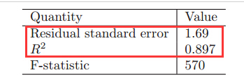
For the Advertising data, the RSE is 1,681units while the mean value for the response is 14,022, indicating a percentage error of roughly 12 %(RSE/mean value). Second, the R2 statistic records the percentage of variability in the response that is explained
by the predictors. The predictors explain almost 90 % of the variance in sales. 



背景知识：
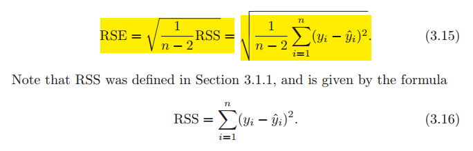
RSE标准差



R2 Statistic（R-square）用于评判一个模型拟合好坏的重要标准
R平方介于0~1之间，越接近1，回归拟合效果越好，模型越精确。

R^2判定系数就是拟合优度判定系数，它体现了回归模型中自变量Y的变异在因变量X的变异中所占的比例。即用来表示y值中有多少可以用x值来解释（R2 measures the proportion

of variability in Y that can be explained using X.），0.92的意思就是y值中有92%可以用x值来解释。
当R^2=1时表示，所有观测点都落在拟合的直线或曲线上；当R^2=0时，表示自变量与因变量不存在直线或曲线关系。

如何根据R-squared判断模型是否准确？
However, it can  still be challenging to determine what is a good R2 value, and in general,  this will depend on the application. For instance, in certain problems in 
physics, we may know that the data truly comes from a linear model with  a small residual error. In this case, we would expect to see an R2 value that is extremely close to 1, and a substantially smaller R2 value might indicate a serious problem with the
experiment in which the data were generated. On the other hand, in typical applications in biology, psychology, marketing, and other domains, the linear model (3.5) is at best an extremely rough approximation to the data, and residual errors due to other unmeasured factors
are often very large. In this setting, we would expect only a very small proportion of the variance in the response to be explained by the 
predictor, and an R2 value well below 0.1 might be more realistic!

4.应用模型：Y准确度（置信度，置信区间，预测区间）

Given a set of predictor values, what response value should we predict, and how accurate is our prediction?
Once we have fit the multiple regression model, it is straightforward to apply  in order to predict the response Y on the basis of a set of values for the predictors X1, X2, . . . , Xp. 

We can compute a confidence interval （置信区间）in order to determine how close Y'(用模型计算出的值) will be to f(X)（理论中的真实值）.
predict an individual response use prediction interval, predict the average response use confidence interval.



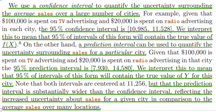
confidence interval置信区间 与预测区间

1 置信区间
表示在给定预测变量的指定设置时，平均响应可能落入的范围。 

置信区间是结合置信度来说的，简单来说就是随机变量有一定概率落在一个范围内，这个概率就叫置信度，范围就是对应的置信区间。
真实数据往往是实际上不能获知的，我们只能进行估计，估计的结果是给出一对数据，比如从1到1.5，真实的值落在1到1.5之间的可能性是95%（也有5%的可能性在这区间之外的）。
90%置信区间（Confidence Interval,CI）：当给出某个估计值的90%置信区间为【a,b】时，可以理解为我们有90%的信心（Confidence）可以说样本的平均值介于a到b之间，而发生错误的概率为10%。 
2 预测区间Prediction Interval
表示在给定预测变量的指定设置时，单个观测值可能落入的范围。

预测区间PI总是要比对应的置信区间CI大，这是因为在对单个响应与响应均值的预测中包括了更多的不确定性。

The basic syntax is lm(y∼x,data), where y is the response（预测值）, x is the predictor（影响因子：x1,x2）, and data is the data set in which these two variables are kept.

5.模型修正

1）各自变量X1，X2...对因变量Y的影响 程度

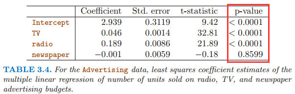
Which media contribute to sales?
To answer this question, we can examine the p-values associated with  each predictor’s t-statistic. In the multiple linear regression displayed in Table 3.4, the p-values for TV and radio are low,but the p-value for newspaper is not. This suggests that
only TV and radio are related to sales. 

2）解决共线性问题

所谓多重共线性（Multicollinearity）是指线性回归模型中的解释变量之间由于存在精确相关关系或高度相关关系而使模型估计失真或难以估计准确。一般来说，由于经济数据的限制使得模型设计不当，导致设计矩阵中解释变量间存在普遍的相关关系。

如何解决共线性问题？
方差膨胀因子（Variance Inflation Factor，VIF）：容忍度的倒数，VIF越大，显示共线性越严重。经验判断方法表明：当0＜VIF＜10，不存在多重共线性；当10≤VIF＜100，存在较强的多重共线性；当VIF≥100，存在严重多重共线性。

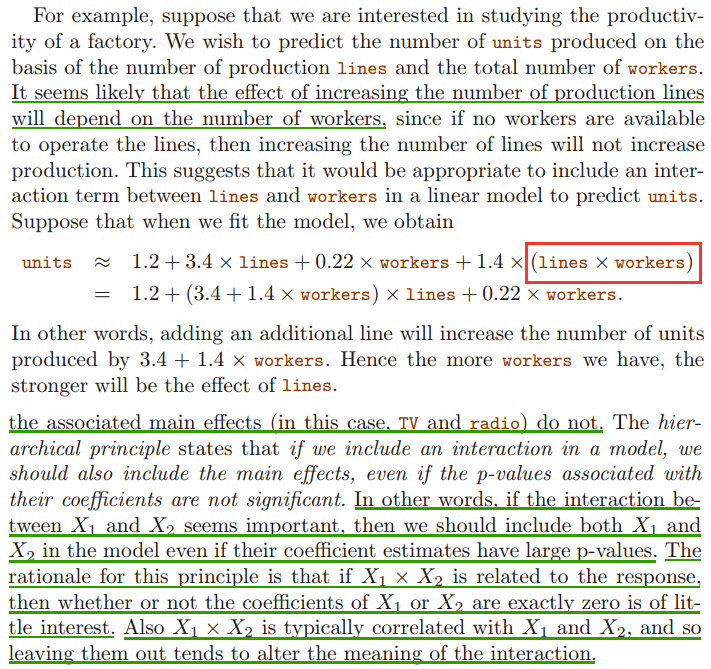
3）交互项系数（interaction terms）

衡量的是一个变量对于“另一个变量对因变量影响能力”的影响。
Is there synergy among the advertising media?
Perhaps spending $50,000 on television advertising and $50,000 on  radio advertising results in more sales than allocating $100,000 to either television or radio individually. In marketing, this is known as 
a synergy effect, while in statistics it is called an interaction effect.

何时适合在模型中加入交互系数？

4）异常值outlier检测

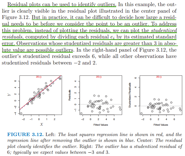
Residual plots（残差散点图） can be used to identify outliers. 检测到异常值后，从数据中去掉异常值，再生成纠正后的模型。

残差是指观测值与预测值（拟合值）之间的差，即是实际观察值与回归估计值的差。 残差分析就是通过残差所提供的信息，分析出数据的可靠性、周期性或其它干扰。在线性回归中,残差的重要应用之一是根据它的绝对值大小判定异常点。
But in practice, it can be difficult to decide how large a residual needs to be before we consider the point to be an outlier. To address this problem, instead of plotting the residuals, we can plot the studentized residuals, computed by dividing each
residual ei by its estimated standard studentized error. Observations whose studentized residuals are greater than 3 in abso- residuallute value are possible outliers.