Python数据分析及可视化的基本环境
2015-05-17 20:39
627 查看
首先搭建基本环境,假设已经有Python运行环境。然后需要装上一些通用的基本库,如numpy, scipy用以数值计算,pandas用以数据分析,matplotlib/Bokeh/Seaborn用来数据可视化。再按需装上数据获取的库,如Tushare(http://pythonhosted.org/tushare/),Quandl(https://www.quandl.com/)等。网上还有很多可供分析的免费数据集(http://www.kdnuggets.com/datasets/index.html)。另外,最好装上IPython,比默认Python
shell强大许多。
更方便地,可以用Anaconda这样的Python发行版,它里面包含了近200个流行的包。从http://continuum.io/downloads选择所用平台的安装包安装。还觉得麻烦的话用Python Quant Platform。Anaconda装好后进入IPython应该就可以看到相关信息了。
下面以一些财经数据为例举一些非常trivial的例子:
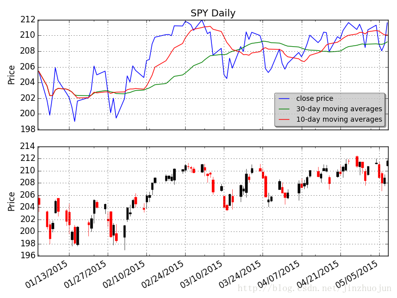
1. SPY的均线和candlestick图
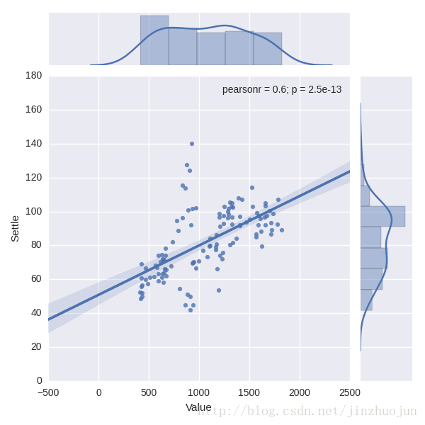
2. 近十年中纽约商业交易所(NYMEX)原油期货价格和黄金价格的线性回归关系
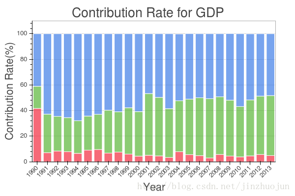
3. 我国三大产业对于GDP的影响
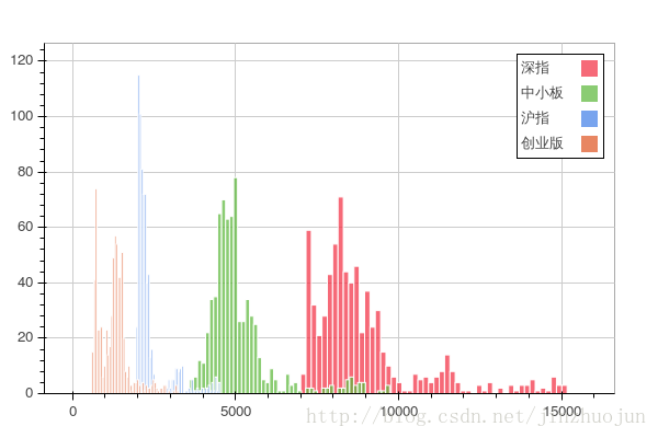
4. 国内沪指,深指等几大指数分布
# -*- coding: utf-8 -*-
from __future__ import unicode_literals
from __future__ import print_function, division
from collections import OrderedDict
import pandas as pd
import tushare as ts
from bokeh.charts import Histogram, output_file, show
sh = ts.get_hist_data('sh')
sz = ts.get_hist_data('sz')
zxb = ts.get_hist_data('zxb')
cyb = ts.get_hist_data('cyb')
df = pd.concat([sh['close'], sz['close'], zxb['close'], cyb['close']], \
axis=1, keys=['sh', 'sz', 'zxb', 'cyb'])
fst_idx = -700
distributions = OrderedDict(sh=list(sh['close'][fst_idx:]), cyb=list(cyb['close'][fst_idx:]), sz=list(sz['close'][fst_idx:]), zxb=list(zxb['close'][fst_idx:]))
df = pd.DataFrame(distributions)
col_mapping = {'sh': u'沪指',
'zxb': u'中小板',
'cyb': u'创业版',
'sz': u'深指'}
df.rename(columns=col_mapping, inplace=True)
output_file("histograms.html")
hist = Histogram(df, bins=50, density=False, legend="top_right")
show(hist)
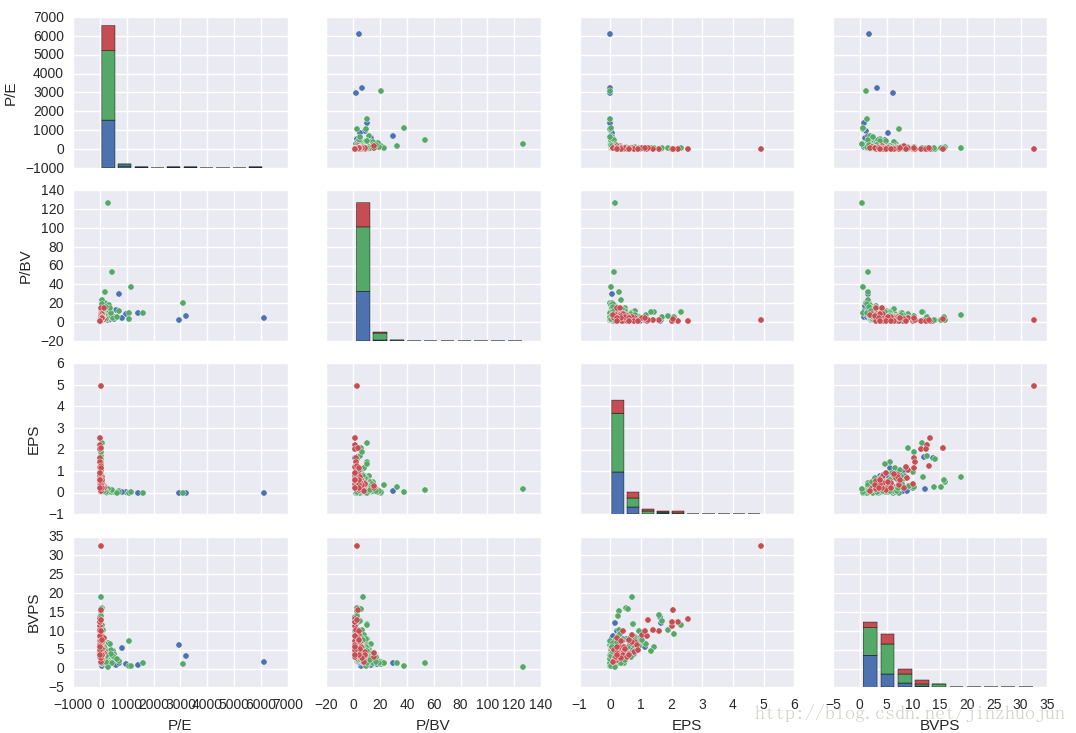
5. 选取某三个行业中上市公司若干关键指标(市盈率,市净率等)的相关性
# -*- coding: utf-8 -*-
from __future__ import print_function, division
from __future__ import unicode_literals
from collections import OrderedDict
import numpy as np
import pandas as pd
import datetime as dt
import seaborn as sns
import tushare as ts
from bokeh.charts import Bar, output_file, show
cls = ts.get_industry_classified()
stk = ts.get_stock_basics()
cls = cls.set_index('code')
tcls = cls[['c_name']]
tstk = stk[['pe', 'pb', 'esp', 'bvps']]
df = tcls.join(tstk, how='inner')
clist = [df.ix[i]['c_name'] for i in xrange(3)]
def neq(a, b, eps=1e-6):
return abs(a - b) > eps
tdf = df.loc[df['c_name'].isin(clist) & neq(df['pe'], 0.0) & \
neq(df['pb'], 0.0) & neq(df['esp'], 0.0) & \
neq(df['bvps'], 0.0)]
col_mapping = {'pe' : u'P/E',
'pb' : u'P/BV',
'esp' : u'EPS',
'bvps' : u'BVPS'}
tdf.rename(columns=col_mapping, inplace=True)
sns.pairplot(tdf, hue='c_name', size=2.5)
shell强大许多。
更方便地,可以用Anaconda这样的Python发行版,它里面包含了近200个流行的包。从http://continuum.io/downloads选择所用平台的安装包安装。还觉得麻烦的话用Python Quant Platform。Anaconda装好后进入IPython应该就可以看到相关信息了。
jzj@jzj-VirtualBox:~/workspace$ ipython
Python 2.7.9 |Anaconda 2.2.0 (64-bit)| (default, Apr 14 2015, 12:54:25)
Type "copyright", "credits" or "license" for more information.

IPython 3.0.0 -- An enhanced Interactive Python.
Anaconda is brought to you by Continuum Analytics.
Please check out: http://continuum.io/thanks and https://binstar.org ...
Anaconda带的conda是一个开源包管理器,可以用conda info/list/search查看信息和已安装包。要安装/更新/删除包可以用conda install/update/remove命令。如:
$ conda install Quandl
$ conda install bokeh
$ conda update pandas
如果还需要装些其它库,比如github上的Python库,可以用Python的包安装方式,如pip install和python setup.py --install。不过要注意的是Anaconda安装路径是独立于原系统中的Python环境的。所以要把包安装到Anaconda那个Python环境的话需要指定下参数,可以先看下Python的包路径:
$ python -m site --user-site然后安装包时指定到该路径,如:
$ python setup.py install --prefix=~/.local如果想避免每次开始工作前都输一坨东西,可以建ipython的profile,在其中进行设置。这样每次ipython启动该profile时,相应的环境都自己设置好了。创建名为work的profile:
$ ipython profile create work然后打开配置文件~/.ipython/profile_work/ipython_config.py,按具体的需求进行修改,比如自动加载一些常用的包。
c.InteractiveShellApp.pylab = 'auto'
...
c.TerminalIPythonApp.exec_lines = [
'import numpy as np',
'import pandas as pd'
...
]
如果大多数时候都要到该profile下工作的话可以在~/.bashrc里加上下面语句:
alias ipython='ipython --profile=work'这样以后只要敲ipython就OK了。进入ipython shell后要运行python脚本只需执行%run test.py。
下面以一些财经数据为例举一些非常trivial的例子:
1. SPY的均线和candlestick图
from __future__ import print_function, division
import numpy as np
import pandas as pd
import datetime as dt
import pandas.io.data as web
import matplotlib.finance as mpf
import matplotlib.dates as mdates
import matplotlib.mlab as mlab
import matplotlib.pyplot as plt
import matplotlib.font_manager as font_manager

starttime = dt.date(2015,1,1)
endtime = dt.date.today()
ticker = 'SPY'

fh = mpf.fetch_historical_yahoo(ticker, starttime, endtime)

r = mlab.csv2rec(fh); fh.close()
r.sort()

df = pd.DataFrame.from_records(r)

quotes = mpf.quotes_historical_yahoo_ohlc(ticker, starttime, endtime)

fig, (ax1, ax2) = plt.subplots(2, sharex=True)

tdf = df.set_index('date')
cdf = tdf['close']
cdf.plot(label = "close price", ax=ax1)
pd.rolling_mean(cdf, window=30, min_periods=1).plot(label = "30-day moving averages", ax=ax1)
pd.rolling_mean(cdf, window=10, min_periods=1).plot(label = "10-day moving averages", ax=ax1)
ax1.set_xlabel(r'Date')
ax1.set_ylabel(r'Price')
ax1.grid(True)
props = font_manager.FontProperties(size=10)
leg = ax1.legend(loc='lower right', shadow=True, fancybox=True, prop=props)
leg.get_frame().set_alpha(0.5)
ax1.set_title('%s Daily' % ticker, fontsize=14)

mpf.candlestick_ohlc(ax2, quotes, width=0.6)
ax2.set_ylabel(r'Price')

for ax in ax1, ax2:
fmt = mdates.DateFormatter('%m/%d/%Y')
ax.xaxis.set_major_formatter(fmt)
ax.grid(True)
ax.xaxis_date()
ax.autoscale()

fig.autofmt_xdate()
fig.tight_layout()
plt.setp(plt.gca().get_xticklabels(), rotation=30)
plt.show()

fig.savefig('SPY.png')
2. 近十年中纽约商业交易所(NYMEX)原油期货价格和黄金价格的线性回归关系
from __future__ import print_function, division
import numpy as np
import pandas as pd
import datetime as dt

import Quandl
import seaborn as sns

sns.set(style="darkgrid")

token = "???" # Notice: You can get the token by signing up on Quandl (https://www.quandl.com/)
starttime = "2005-01-01"
endtime = "2015-01-01"
interval = "monthly"

gold = Quandl.get("BUNDESBANK/BBK01_WT5511", authtoken=token, trim_start=starttime, trim_end=endtime, collapse=interval)
nymex_oil_future = Quandl.get("OFDP/FUTURE_CL1", authtoken=token, trim_start=starttime, trim_end=endtime, collapse=interval)
brent_oil_future = Quandl.get("CHRIS/ICE_B1", authtoken=token, trim_start=starttime, trim_end=endtime, collapse=interval)

#dat = nymex_oil_future.join(brent_oil_future, lsuffix='_a', rsuffix='_b', how='inner')
#g = sns.jointplot("Settle_a", "Settle_b", data=dat, kind="reg")

dat = gold.join(nymex_oil_future, lsuffix='_a', rsuffix='_b', how='inner')
g = sns.jointplot("Value", "Settle", data=dat, kind="reg")
3. 我国三大产业对于GDP的影响
from __future__ import print_function, division
from collections import OrderedDict

import numpy as np
import pandas as pd
import datetime as dt

import tushare as ts
from bokeh.charts import Bar, output_file, show
import bokeh.plotting as bp

df = ts.get_gdp_contrib()
df = df.drop(['industry', 'gdp_yoy'], axis=1)
df = df.set_index('year')
df = df.sort_index()

years = df.index.values.tolist()

pri = df['pi'].astype(float).values
sec = df['si'].astype(float).values
ter = df['ti'].astype(float).values

contrib = OrderedDict(Primary=pri, Secondary=sec, Tertiary=ter)
years = map(unicode, map(str, years))

output_file("stacked_bar.html")
bar = Bar(contrib, years, stacked=True, title="Contribution Rate for GDP", \
xlabel="Year", ylabel="Contribution Rate(%)")
show(bar)
4. 国内沪指,深指等几大指数分布
# -*- coding: utf-8 -*-
from __future__ import unicode_literals
from __future__ import print_function, division
from collections import OrderedDict
import pandas as pd
import tushare as ts
from bokeh.charts import Histogram, output_file, show
sh = ts.get_hist_data('sh')
sz = ts.get_hist_data('sz')
zxb = ts.get_hist_data('zxb')
cyb = ts.get_hist_data('cyb')
df = pd.concat([sh['close'], sz['close'], zxb['close'], cyb['close']], \
axis=1, keys=['sh', 'sz', 'zxb', 'cyb'])
fst_idx = -700
distributions = OrderedDict(sh=list(sh['close'][fst_idx:]), cyb=list(cyb['close'][fst_idx:]), sz=list(sz['close'][fst_idx:]), zxb=list(zxb['close'][fst_idx:]))
df = pd.DataFrame(distributions)
col_mapping = {'sh': u'沪指',
'zxb': u'中小板',
'cyb': u'创业版',
'sz': u'深指'}
df.rename(columns=col_mapping, inplace=True)
output_file("histograms.html")
hist = Histogram(df, bins=50, density=False, legend="top_right")
show(hist)
5. 选取某三个行业中上市公司若干关键指标(市盈率,市净率等)的相关性
# -*- coding: utf-8 -*-
from __future__ import print_function, division
from __future__ import unicode_literals
from collections import OrderedDict
import numpy as np
import pandas as pd
import datetime as dt
import seaborn as sns
import tushare as ts
from bokeh.charts import Bar, output_file, show
cls = ts.get_industry_classified()
stk = ts.get_stock_basics()
cls = cls.set_index('code')
tcls = cls[['c_name']]
tstk = stk[['pe', 'pb', 'esp', 'bvps']]
df = tcls.join(tstk, how='inner')
clist = [df.ix[i]['c_name'] for i in xrange(3)]
def neq(a, b, eps=1e-6):
return abs(a - b) > eps
tdf = df.loc[df['c_name'].isin(clist) & neq(df['pe'], 0.0) & \
neq(df['pb'], 0.0) & neq(df['esp'], 0.0) & \
neq(df['bvps'], 0.0)]
col_mapping = {'pe' : u'P/E',
'pb' : u'P/BV',
'esp' : u'EPS',
'bvps' : u'BVPS'}
tdf.rename(columns=col_mapping, inplace=True)
sns.pairplot(tdf, hue='c_name', size=2.5)

相关文章推荐
- Caffe学习系列(13):数据可视化环境(python接口)配置
- 用python做数据分析4|pandas库介绍之DataFrame基本操作
- Caffe学习系列:数据可视化环境(python接口)配置
- Caffe学习系列(13):数据可视化环境(python接口)配置
- 利用Python对NBA SportUV数据进行可视化及分析
- Python爬虫实现数据可视化,为你做一个城市旅游数据分析
- Python数据分析模块 | pandas做数据分析(一):基本数据对象
- 在MAC上搭建python数据分析开发环境
- 利用Python进行数据分析——第8章绘图及可视化——学习笔记Python3 5.0.0
- 分析python处理基本数据<二>
- 利用Python进行数据分析环境部署
- Caffe学习系列(11):数据可视化环境(python接口)配置
- Python 数据分析(一) 本实验将学习 pandas 基础,数据加载、存储与文件格式,数据规整化,绘图和可视化的知识
- 利用Python进行数据分析--绘图和可视化
- python数据分析(数据可视化)
- Python数据可视化图像库MatPlotLib基本图像操作
- Python数据分析库pandas基本操作
- python数据分析之:绘图和可视化
- 基于Python的数据分析(1):配置安装环境
- 用python做数据分析4|pandas库介绍之DataFrame基本操作