matlab线性拟合与曲线拟合
2013-04-01 16:42
621 查看
使用Matlab进行拟合是图像处理中线条变换的一个重点内容,本文将详解Matlab中的直线拟合和曲线拟合用法。
关键函数:
ffun = fittype(expr)
ffun = fittype({expr1,...,exprn})
ffun = fittype(expr, Name, Value,...)
ffun= fittype({expr1,...,exprn}, Name, Value,...)
/***********************************线性拟合***********************************/
线性拟合公式:
线性拟合Example:
Example1: y=kx+b;
法1:
[csharp]
view plaincopyprint?
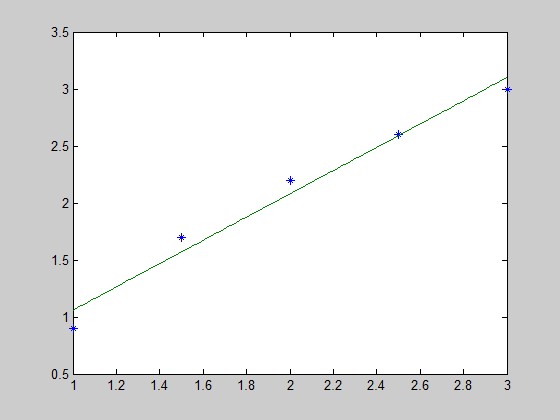
x=[1,1.5,2,2.5,3];y=[0.9,1.7,2.2,2.6,3];
p=polyfit(x,y,1);
x1=linspace(min(x),max(x));
y1=polyval(p,x1);
plot(x,y,'*',x1,y1);
即y=1.0200 *x+ 0.0400
法2:
[csharp]
view plaincopyprint?
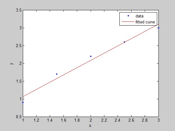
x=[1;1.5;2;2.5;3];y=[0.9;1.7;2.2;2.6;3];
p=fittype('poly1')
f=fit(x,y,p)
plot(f,x,y);
[csharp]
view plaincopyprint?
 x=[1;1.5;2;2.5;3];y=[0.9;1.7;2.2;2.6;3];
p=fittype('poly1')
f=fit(x,y,p)
plot(f,x,y);

p =

Linear model Poly1:
p(p1,p2,x) = p1*x + p2

f =

Linear model Poly1:
f(x) = p1*x + p2
Coefficients (with 95% confidence bounds):
p1 =        1.02  (0.7192, 1.321)
p2 =        0.04  (-0.5981, 0.6781)
Example2:y=a*x + b*sin(x) + c
法1:
[csharp]
view plaincopyprint?
x=[1;1.5;2;2.5;3];y=[0.9;1.7;2.2;2.6;3];
EXPR = {'x','sin(x)','1'};
p=fittype(EXPR)
f=fit(x,y,p)
plot(f,x,y);
运行结果:
[csharp]
view plaincopyprint?
 x=[1;1.5;2;2.5;3];y=[0.9;1.7;2.2;2.6;3];
EXPR = {'x','sin(x)','1'};
p=fittype(EXPR)
f=fit(x,y,p)
plot(f,x,y);

p =

Linear model:
p(a,b,c,x) = a*x + b*sin(x) + c

f =

Linear model:
f(x) = a*x + b*sin(x) + c
Coefficients (with 95% confidence bounds):
a =       1.249  (0.9856, 1.512)
b =      0.6357  (0.03185, 1.24)
c =     -0.8611  (-1.773, 0.05094)
法2:
[csharp]
view plaincopyprint?
x=[1;1.5;2;2.5;3];y=[0.9;1.7;2.2;2.6;3];
p=fittype('a*x+b*sin(x)+c','independent','x')
f=fit(x,y,p)
plot(f,x,y);
运行结果:
[csharp]
view plaincopyprint?
x=[1;1.5;2;2.5;3];y=[0.9;1.7;2.2;2.6;3];
p=fittype('a*x+b*sin(x)+c','independent','x')
f=fit(x,y,p)
plot(f,x,y);

p =

General model:
p(a,b,c,x) = a*x+b*sin(x)+c
Warning: Start point not provided, choosing random start
point.
> In fit>iCreateWarningFunction/nThrowWarning at 738
In fit>iFit at 320
In fit at 109

f =

General model:
f(x) = a*x+b*sin(x)+c
Coefficients (with 95% confidence bounds):
a =       1.249  (0.9856, 1.512)
b =      0.6357  (0.03185, 1.24)
c =     -0.8611  (-1.773, 0.05094)

/***********************************非线性拟合***********************************/
Example:y=a*x^2+b*x+c
法1:
[cpp]
view plaincopyprint?
x=[1;1.5;2;2.5;3];y=[0.9;1.7;2.2;2.6;3];
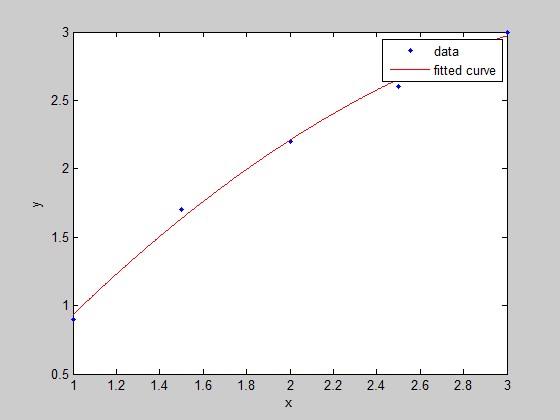
p=fittype('a*x.^2+b*x+c','independent','x')
f=fit(x,y,p)
plot(f,x,y);
运行结果:
[csharp]
view plaincopyprint?
p =

General model:
p(a,b,c,x) = a*x.^2+b*x+c
Warning: Start point not provided, choosing random start
point.
> In fit>iCreateWarningFunction/nThrowWarning at 738
In fit>iFit at 320
In fit at 109

f =

General model:
f(x) = a*x.^2+b*x+c
Coefficients (with 95% confidence bounds):
a =     -0.2571  (-0.5681, 0.05386)
b =       2.049  (0.791, 3.306)
c =       -0.86  (-2.016, 0.2964)
法2:
[csharp]
view plaincopyprint?
x=[1;1.5;2;2.5;3];y=[0.9;1.7;2.2;2.6;3];
%use c=0;
c=0;
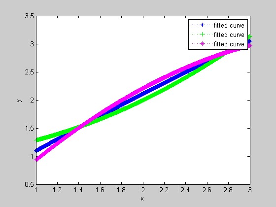
p1=fittype(@(a,b,x) a*x.^2+b*x+c)
f1=fit(x,y,p1)
%use c=1;
c=1;
p2=fittype(@(a,b,x) a*x.^2+b*x+c)
f2=fit(x,y,p2)
%predict c
p3=fittype(@(a,b,c,x) a*x.^2+b*x+c)
f3=fit(x,y,p3)
%show results
scatter(x,y);%scatter point
c1=plot(f1,'b:*');%blue
hold on
plot(f2,'g:+');%green
hold on
plot(f3,'m:*');%purple
hold off
关键函数:
fittype
Fit type for curve and surface fittingSyntax
ffun = fittype(libname)ffun = fittype(expr)
ffun = fittype({expr1,...,exprn})
ffun = fittype(expr, Name, Value,...)
ffun= fittype({expr1,...,exprn}, Name, Value,...)
/***********************************线性拟合***********************************/
线性拟合公式:
coeff1 * term1 + coeff2 * term2 + coeff3 * term3 + ...其中,coefficient是系数,term都是x的一次项。
线性拟合Example:
Example1: y=kx+b;
法1:
[csharp]
view plaincopyprint?
x=[1,1.5,2,2.5,3];y=[0.9,1.7,2.2,2.6,3]; p=polyfit(x,y,1); x1=linspace(min(x),max(x)); y1=polyval(p,x1); plot(x,y,'*',x1,y1);
x=[1,1.5,2,2.5,3];y=[0.9,1.7,2.2,2.6,3]; p=polyfit(x,y,1); x1=linspace(min(x),max(x)); y1=polyval(p,x1); plot(x,y,'*',x1,y1);结果:p = 1.0200 0.0400
即y=1.0200 *x+ 0.0400
法2:
[csharp]
view plaincopyprint?
x=[1;1.5;2;2.5;3];y=[0.9;1.7;2.2;2.6;3]; p=fittype('poly1') f=fit(x,y,p) plot(f,x,y);
x=[1;1.5;2;2.5;3];y=[0.9;1.7;2.2;2.6;3];
p=fittype('poly1')
f=fit(x,y,p)
plot(f,x,y);运行结果:[csharp]
view plaincopyprint?
x=[1;1.5;2;2.5;3];y=[0.9;1.7;2.2;2.6;3]; p=fittype('poly1') f=fit(x,y,p) plot(f,x,y);
p =
Linear model Poly1:
p(p1,p2,x) = p1*x + p2
f =
Linear model Poly1:
f(x) = p1*x + p2
Coefficients (with 95% confidence bounds):
p1 = 1.02 (0.7192, 1.321)
p2 = 0.04 (-0.5981, 0.6781)
x=[1;1.5;2;2.5;3];y=[0.9;1.7;2.2;2.6;3];
p=fittype('poly1')
f=fit(x,y,p)
plot(f,x,y);
p =
Linear model Poly1:
p(p1,p2,x) = p1*x + p2
f =
Linear model Poly1:
f(x) = p1*x + p2
Coefficients (with 95% confidence bounds):
p1 = 1.02 (0.7192, 1.321)
p2 = 0.04 (-0.5981, 0.6781)Example2:y=a*x + b*sin(x) + c
法1:
[csharp]
view plaincopyprint?
x=[1;1.5;2;2.5;3];y=[0.9;1.7;2.2;2.6;3]; EXPR = {'x','sin(x)','1'}; p=fittype(EXPR) f=fit(x,y,p) plot(f,x,y);
x=[1;1.5;2;2.5;3];y=[0.9;1.7;2.2;2.6;3];
EXPR = {'x','sin(x)','1'};
p=fittype(EXPR)
f=fit(x,y,p)
plot(f,x,y);运行结果:
[csharp]
view plaincopyprint?
x=[1;1.5;2;2.5;3];y=[0.9;1.7;2.2;2.6;3]; EXPR = {'x','sin(x)','1'}; p=fittype(EXPR) f=fit(x,y,p) plot(f,x,y);
p =
Linear model:
p(a,b,c,x) = a*x + b*sin(x) + c
f =
Linear model:
f(x) = a*x + b*sin(x) + c
Coefficients (with 95% confidence bounds):
a = 1.249 (0.9856, 1.512)
b = 0.6357 (0.03185, 1.24)
c = -0.8611 (-1.773, 0.05094)
x=[1;1.5;2;2.5;3];y=[0.9;1.7;2.2;2.6;3];
EXPR = {'x','sin(x)','1'};
p=fittype(EXPR)
f=fit(x,y,p)
plot(f,x,y);
p =
Linear model:
p(a,b,c,x) = a*x + b*sin(x) + c
f =
Linear model:
f(x) = a*x + b*sin(x) + c
Coefficients (with 95% confidence bounds):
a = 1.249 (0.9856, 1.512)
b = 0.6357 (0.03185, 1.24)
c = -0.8611 (-1.773, 0.05094)法2:
[csharp]
view plaincopyprint?
x=[1;1.5;2;2.5;3];y=[0.9;1.7;2.2;2.6;3];
p=fittype('a*x+b*sin(x)+c','independent','x')
f=fit(x,y,p)
plot(f,x,y);
x=[1;1.5;2;2.5;3];y=[0.9;1.7;2.2;2.6;3];
p=fittype('a*x+b*sin(x)+c','independent','x')
f=fit(x,y,p)
plot(f,x,y);运行结果:
[csharp]
view plaincopyprint?
x=[1;1.5;2;2.5;3];y=[0.9;1.7;2.2;2.6;3];
p=fittype('a*x+b*sin(x)+c','independent','x')
f=fit(x,y,p)
plot(f,x,y);
p =
General model:
p(a,b,c,x) = a*x+b*sin(x)+c
Warning: Start point not provided, choosing random start
point.
> In fit>iCreateWarningFunction/nThrowWarning at 738
In fit>iFit at 320
In fit at 109
f =
General model:
f(x) = a*x+b*sin(x)+c
Coefficients (with 95% confidence bounds):
a = 1.249 (0.9856, 1.512)
b = 0.6357 (0.03185, 1.24)
c = -0.8611 (-1.773, 0.05094)
x=[1;1.5;2;2.5;3];y=[0.9;1.7;2.2;2.6;3];
p=fittype('a*x+b*sin(x)+c','independent','x')
f=fit(x,y,p)
plot(f,x,y);
p =
General model:
p(a,b,c,x) = a*x+b*sin(x)+c
Warning: Start point not provided, choosing random start
point.
> In fit>iCreateWarningFunction/nThrowWarning at 738
In fit>iFit at 320
In fit at 109
f =
General model:
f(x) = a*x+b*sin(x)+c
Coefficients (with 95% confidence bounds):
a = 1.249 (0.9856, 1.512)
b = 0.6357 (0.03185, 1.24)
c = -0.8611 (-1.773, 0.05094)/***********************************非线性拟合***********************************/
Example:y=a*x^2+b*x+c
法1:
[cpp]
view plaincopyprint?
x=[1;1.5;2;2.5;3];y=[0.9;1.7;2.2;2.6;3];
p=fittype('a*x.^2+b*x+c','independent','x')
f=fit(x,y,p)
plot(f,x,y);
x=[1;1.5;2;2.5;3];y=[0.9;1.7;2.2;2.6;3];
p=fittype('a*x.^2+b*x+c','independent','x')
f=fit(x,y,p)
plot(f,x,y);运行结果:
[csharp]
view plaincopyprint?
p =
General model:
p(a,b,c,x) = a*x.^2+b*x+c
Warning: Start point not provided, choosing random start
point.
> In fit>iCreateWarningFunction/nThrowWarning at 738
In fit>iFit at 320
In fit at 109
f =
General model:
f(x) = a*x.^2+b*x+c
Coefficients (with 95% confidence bounds):
a = -0.2571 (-0.5681, 0.05386)
b = 2.049 (0.791, 3.306)
c = -0.86 (-2.016, 0.2964)
p = General model: p(a,b,c,x) = a*x.^2+b*x+c Warning: Start point not provided, choosing random start point. > In fit>iCreateWarningFunction/nThrowWarning at 738 In fit>iFit at 320 In fit at 109 f = General model: f(x) = a*x.^2+b*x+c Coefficients (with 95% confidence bounds): a = -0.2571 (-0.5681, 0.05386) b = 2.049 (0.791, 3.306) c = -0.86 (-2.016, 0.2964)
法2:
[csharp]
view plaincopyprint?
x=[1;1.5;2;2.5;3];y=[0.9;1.7;2.2;2.6;3];
%use c=0;
c=0;
p1=fittype(@(a,b,x) a*x.^2+b*x+c)
f1=fit(x,y,p1)
%use c=1;
c=1;
p2=fittype(@(a,b,x) a*x.^2+b*x+c)
f2=fit(x,y,p2)
%predict c
p3=fittype(@(a,b,c,x) a*x.^2+b*x+c)
f3=fit(x,y,p3)
%show results
scatter(x,y);%scatter point
c1=plot(f1,'b:*');%blue
hold on
plot(f2,'g:+');%green
hold on
plot(f3,'m:*');%purple
hold off
x=[1;1.5;2;2.5;3];y=[0.9;1.7;2.2;2.6;3]; %use c=0; c=0; p1=fittype(@(a,b,x) a*x.^2+b*x+c) f1=fit(x,y,p1) %use c=1; c=1; p2=fittype(@(a,b,x) a*x.^2+b*x+c) f2=fit(x,y,p2) %predict c p3=fittype(@(a,b,c,x) a*x.^2+b*x+c) f3=fit(x,y,p3) %show results scatter(x,y);%scatter point c1=plot(f1,'b:*');%blue hold on plot(f2,'g:+');%green hold on plot(f3,'m:*');%purple hold off

相关文章推荐
- matlab 万能实用的线性曲线拟合方法
- Matlab的曲线拟合工具箱CFtool使用简介
- Matlab曲线拟合函数
- Matlab 线性拟合 & 非线性拟合
- Matlab 线性拟合 & 非线性拟合
- matlab 曲线拟合--视频编码中PSNR计算及码率计算(1)
- Matlab曲线拟合
- 用matlab实现非线性曲线拟合
- Matlab单一变量曲线拟合-cftool
- MATLAB 线性拟合 决定系数R2求解
- Matlab曲线拟合
- matlab曲线拟合
- matlab曲线拟合工具箱cftool
- Matlab曲线拟合工具箱
- matlab曲线拟合 函数 用法以及例子
- matlab 曲线拟合工具箱 cftool
- MATLAB利用散点进行函数曲线拟合
- matlab进行离散点的曲线拟合
- Matlab拟合曲线之幂律分布
- matlab中的曲线拟合与插值