AI 基础：Scipy（科学计算库） 简易入门

0.导语

Scipy是一个用于数学、科学、工程领域的常用软件包，可以处理插值、积分、优化、图像处理、常微分方程数值解的求解、信号处理等问题。它用于有效计算Numpy矩阵，使Numpy和Scipy协同工作，高效解决问题。

Scipy是由针对特定任务的子模块组成：

在此之前，我已经写了以下几篇AI基础的快速入门，本篇文章讲解科学计算库Scipy快速入门：

已发布：

AI 基础：Numpy 简易入门

AI 基础：Pandas 简易入门

AI基础：数据可视化简易入门（matplotlib和seaborn）

备注：本文代码可以在github下载

https://github.com/fengdu78/Data-Science-Notes/tree/master/4.scipy

1.SciPy-数值计算库

import numpy as np
import pylab as pl

import matplotlib as mpl
mpl.rcParams['font.sans-serif'] = ['SimHei']

import scipy
scipy.__version__#查看版本

'1.0.0'

常数和特殊函数

from scipy import constants as C
print (C.c) # 真空中的光速
print (C.h) # 普朗克常数

299792458.0
6.62607004e-34

C.physical_constants["electron mass"]

(9.10938356e-31, 'kg', 1.1e-38)

# 1英里等于多少米, 1英寸等于多少米, 1克等于多少千克, 1磅等于多少千克
print(C.mile)
print(C.inch)
print(C.gram)
print(C.pound)

1609.3439999999998
0.0254
0.001
0.45359236999999997

import scipy.special as S

print (1 + 1e-20)
print (np.log(1+1e-20))
print (S.log1p(1e-20))

1.0
0.0
1e-20

m = np.linspace(0.1, 0.9, 4)
u = np.linspace(-10, 10, 200)
results = S.ellipj(u[:, None], m[None, :])

print([y.shape for y in results])

[(200, 4), (200, 4), (200, 4), (200, 4)]

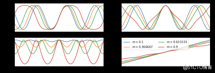
#%figonly=使用广播计算得到的`ellipj()`返回值
fig, axes = pl.subplots(2, 2, figsize=(12, 4))
labels = ["$sn$", "$cn$", "$dn$", "$\phi$"]
for ax, y, label in zip(axes.ravel(), results, labels):
ax.plot(u, y)
ax.set_ylabel(label)
ax.margins(0, 0.1)

axes[1, 1].legend(["$m={:g}$".format(m_) for m_ in m], loc="best", ncol=2);

2.拟合与优化-optimize

非线性方程组求解

import pylab as pl
import numpy as np

import matplotlib as mpl
mpl.rcParams['font.sans-serif'] = ['SimHei']

from math import sin, cos
from scipy import optimize

def f(x): #❶
x0, x1, x2 = x.tolist() #❷
return [
5*x1+3,
4*x0*x0 - 2*sin(x1*x2),
x1*x2 - 1.5
]

# f计算方程组的误差，[1,1,1]是未知数的初始值
result = optimize.fsolve(f, [1,1,1]) #❸
print (result)
print (f(result))

[-0.70622057 -0.6 -2.5 ]
[0.0, -9.126033262418787e-14, 5.329070518200751e-15]

def j(x):  #❶
x0, x1, x2 = x.tolist()
return [[0, 5, 0],
[8 * x0, -2 * x2 * cos(x1 * x2), -2 * x1 * cos(x1 * x2)],
[0, x2, x1]]

result = optimize.fsolve(f, [1, 1, 1], fprime=j)  #❷
print(result)
print(f(result))

[-0.70622057 -0.6 -2.5 ]
[0.0, -9.126033262418787e-14, 5.329070518200751e-15]

最小二乘拟合

import numpy as np
from scipy import optimize

X = np.array([ 8.19,  2.72,  6.39,  8.71,  4.7 ,  2.66,  3.78])
Y = np.array([ 7.01,  2.78,  6.47,  6.71,  4.1 ,  4.23,  4.05])

def residuals(p): #❶
"计算以p为参数的直线和原始数据之间的误差"
k, b = p
return Y - (k*X + b)

# leastsq使得residuals()的输出数组的平方和最小，参数的初始值为[1,0]
r = optimize.leastsq(residuals, [1, 0]) #❷
k, b = r[0]
print ("k =",k, "b =",b)

k = 0.6134953491930442 b = 1.794092543259387

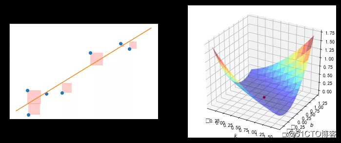
#%figonly=最小化正方形面积之和（左），误差曲面（右）
scale_k = 1.0
scale_b = 10.0
scale_error = 1000.0

def S(k, b):
"计算直线y=k*x+b和原始数据X、Y的误差的平方和"
error = np.zeros(k.shape)
for x, y in zip(X, Y):
error += (y - (k * x + b)) ** 2
return error

ks, bs = np.mgrid[k - scale_k:k + scale_k:40j, b - scale_b:b + scale_b:40j]
error = S(ks, bs) / scale_error

from mpl_toolkits.mplot3d import Axes3D
from matplotlib.patches import Rectangle

fig = pl.figure(figsize=(12, 5))

ax1 = pl.subplot(121)

ax1.plot(X, Y, "o")
X0 = np.linspace(2, 10, 3)
Y0 = k*X0 + b
ax1.plot(X0, Y0)

for x, y in zip(X, Y):
y2 = k*x+b
rect = Rectangle((x,y), abs(y-y2), y2-y, facecolor="red", alpha=0.2)
ax1.add_patch(rect)

ax1.set_aspect("equal")

ax2 = fig.add_subplot(122, projection='3d')

ax2.plot_surface(
ks, bs / scale_b, error, rstride=3, cstride=3, cmap="jet", alpha=0.5)
ax2.scatter([k], [b / scale_b], [S(k, b) / scale_error], c="r", s=20)
ax2.set_xlabel("$k$")
ax2.set_ylabel("$b$")
ax2.set_zlabel("$error$");

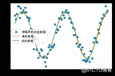
#%fig=带噪声的正弦波拟合
def func(x, p):  #❶
"""
数据拟合所用的函数: A*sin(2*pi*k*x + theta)
"""
A, k, theta = p
return A * np.sin(2 * np.pi * k * x + theta)

def residuals(p, y, x):  #❷
"""
实验数据x, y和拟合函数之间的差，p为拟合需要找到的系数
"""
return y - func(x, p)

x = np.linspace(0, 2 * np.pi, 100)
A, k, theta = 10, 0.34, np.pi / 6  # 真实数据的函数参数
y0 = func(x, [A, k, theta])  # 真实数据
# 加入噪声之后的实验数据
np.random.seed(0)
y1 = y0 + 2 * np.random.randn(len(x))  #❸

p0 = [7, 0.40, 0]  # 第一次猜测的函数拟合参数

# 调用leastsq进行数据拟合
# residuals为计算误差的函数
# p0为拟合参数的初始值
# args为需要拟合的实验数据
plsq = optimize.leastsq(residuals, p0, args=(y1, x))  #❹

print(u"真实参数:", [A, k, theta])
print(u"拟合参数", plsq[0])  # 实验数据拟合后的参数

pl.plot(x, y1, "o", label=u"带噪声的实验数据")
pl.plot(x, y0, label=u"真实数据")
pl.plot(x, func(x, plsq[0]), label=u"拟合数据")
pl.legend(loc="best")

真实参数: [10, 0.34, 0.5235987755982988]
拟合参数 [10.25218748 0.3423992 0.50817423]

def func2(x, A, k, theta):
return A*np.sin(2*np.pi*k*x+theta)

popt, _ = optimize.curve_fit(func2, x, y1, p0=p0)
print (popt)

[10.25218748 0.3423992 0.50817425]

popt, _ = optimize.curve_fit(func2, x, y1, p0=[10, 1, 0])

print(u"真实参数:", [A, k, theta])

print(u"拟合参数", popt)

真实参数: [10, 0.34, 0.5235987755982988]
拟合参数 [ 0.71093469 1.02074585 -0.12776742]

计算函数局域最小值

def target_function(x, y):
return (1 - x)**2 + 100 * (y - x**2)**2

class TargetFunction(object):
def __init__(self):
self.f_points = []
self.fprime_points = []
self.fhess_points = []

def f(self, p):
x, y = p.tolist()
z = target_function(x, y)
self.f_points.append((x, y))
return z

def fprime(self, p):
x, y = p.tolist()
self.fprime_points.append((x, y))
dx = -2 + 2 * x - 400 * x * (y - x**2)
dy = 200 * y - 200 * x**2
return np.array([dx, dy])

def fhess(self, p):
x, y = p.tolist()
self.fhess_points.append((x, y))
return np.array([[2 * (600 * x**2 - 200 * y + 1), -400 * x],
[-400 * x, 200]])

def fmin_demo(method):
target = TargetFunction()
init_point = (-1, -1)
res = optimize.minimize(
target.f,
init_point,
method=method,
jac=target.fprime,
hess=target.fhess)
return res, [
np.array(points) for points in (target.f_points, target.fprime_points,
target.fhess_points)
]

methods = ("Nelder-Mead", "Powell", "CG", "BFGS", "Newton-CG", "L-BFGS-B")
for method in methods:
res, (f_points, fprime_points, fhess_points) = fmin_demo(method)
print(
"{:12s}: min={:12g}, f count={:3d}, fprime count={:3d}, fhess count={:3d}"
.format(method, float(res["fun"]), len(f_points), len(fprime_points),
len(fhess_points)))

Nelder-Mead : min= 5.30934e-10, f count=125, fprime count= 0, fhess count= 0
Powell : min= 0, f count= 52, fprime count= 0, fhess count= 0
CG : min= 9.63056e-21, f count= 39, fprime count= 39, fhess count= 0
BFGS : min= 1.84992e-16, f count= 40, fprime count= 40, fhess count= 0
Newton-CG : min= 5.22666e-10, f count= 60, fprime count= 97, fhess count= 38
L-BFGS-B : min= 6.5215e-15, f count= 33, fprime count= 33, fhess count= 0

#%figonly=各种优化算法的搜索路径
def draw_fmin_demo(f_points, fprime_points, ax):
xmin, xmax = -3, 3
ymin, ymax = -3, 3
Y, X = np.ogrid[ymin:ymax:500j,xmin:xmax:500j]
Z = np.log10(target_function(X, Y))
zmin, zmax = np.min(Z), np.max(Z)
ax.imshow(Z, extent=(xmin,xmax,ymin,ymax), origin="bottom", aspect="auto", cmap="gray")
ax.plot(f_points[:,0], f_points[:,1], lw=1)
ax.scatter(f_points[:,0], f_points[:,1], c=range(len(f_points)), s=50, linewidths=0)
if len(fprime_points):
ax.scatter(fprime_points[:, 0], fprime_points[:, 1], marker="x", color="w", alpha=0.5)
ax.set_xlim(xmin, xmax)
ax.set_ylim(ymin, ymax)

fig, axes = pl.subplots(2, 3, figsize=(9, 6))
methods = ("Nelder-Mead", "Powell", "CG", "BFGS", "Newton-CG", "L-BFGS-B")
for ax, method in zip(axes.ravel(), methods):
res, (f_points, fprime_points, fhess_points) = fmin_demo(method)
draw_fmin_demo(f_points, fprime_points, ax)
ax.set_aspect("equal")
ax.set_title(method)

计算全域最小值

def func(x, p):
A, k, theta = p
return A*np.sin(2*np.pi*k*x+theta)

def func_error(p, y, x):
return np.sum((y - func(x, p))**2)

x = np.linspace(0, 2*np.pi, 100)
A, k, theta = 10, 0.34, np.pi/6
y0 = func(x, [A, k, theta])
np.random.seed(0)
y1 = y0 + 2 * np.random.randn(len(x))

result = optimize.basinhopping(func_error, (1, 1, 1),
niter = 10,
minimizer_kwargs={"method":"L-BFGS-B",
"args":(y1, x)})
print (result.x)

[10.25218676 -0.34239909 2.63341581]

#%figonly=用`basinhopping()`拟合正弦波
pl.plot(x, y1, "o", label=u"带噪声的实验数据")
pl.plot(x, y0, label=u"真实数据")
pl.plot(x, func(x, result.x), label=u"拟合数据")
pl.legend(loc="best");

3.线性代数-linalg

解线性方程组

import pylab as pl
import numpy as np
from scipy import linalg

import matplotlib as mpl
mpl.rcParams['font.sans-serif'] = ['SimHei']

import numpy as np
from scipy import linalg
m, n = 500, 50
A = np.random.rand(m, m)
B = np.random.rand(m, n)
X1 = linalg.solve(A, B)
X2 = np.dot(linalg.inv(A), B)
print (np.allclose(X1, X2))
%timeit linalg.solve(A, B)
%timeit np.dot(linalg.inv(A), B)

True
5.38 ms ± 120 µs per loop (mean ± std. dev. of 7 runs, 100 loops each)
8.14 ms ± 994 µs per loop (mean ± std. dev. of 7 runs, 100 loops each)

luf = linalg.lu_factor(A)
X3 = linalg.lu_solve(luf, B)
np.allclose(X1, X3)

True

M, N = 1000, 100
np.random.seed(0)
A = np.random.rand(M, M)
B = np.random.rand(M, N)
Ai = linalg.inv(A)
luf = linalg.lu_factor(A)
%timeit linalg.inv(A)
%timeit np.dot(Ai, B)
%timeit linalg.lu_factor(A)
%timeit linalg.lu_solve(luf, B)

50.6 ms ± 1.94 ms per loop (mean ± std. dev. of 7 runs, 10 loops each)
3.49 ms ± 306 µs per loop (mean ± std. dev. of 7 runs, 100 loops each)
20.1 ms ± 1.42 ms per loop (mean ± std. dev. of 7 runs, 10 loops each)
4.49 ms ± 65 µs per loop (mean ± std. dev. of 7 runs, 100 loops each)

最小二乘解

from numpy.lib.stride_tricks import as_strided
def make_data(m, n, noise_scale):  #❶
np.random.seed(42)
x = np.random.standard_normal(m)
h = np.random.standard_normal(n)
y = np.convolve(x, h)
yn = y + np.random.standard_normal(len(y)) * noise_scale * np.max(y)
return x, yn, h

def solve_h(x, y, n):  #❷
X = as_strided(
x, shape=(len(x) - n + 1, n), strides=(x.itemsize, x.itemsize))  #❸
Y = y[n - 1:len(x)]  #❹
h = linalg.lstsq(X, Y)  #❺
return h[0][::-1]  #❻

x, yn, h = make_data(1000, 100, 0.4)
H1 = solve_h(x, yn, 120)
H2 = solve_h(x, yn, 80)

print("Average error of H1:", np.mean(np.abs(h[:100] - h)))
print("Average error of H2:", np.mean(np.abs(h[:80] - H2)))

Average error of H1: 0.0
Average error of H2: 0.2958422158342371

#%figonly=实际的系统参数与最小二乘解的比较
fig, (ax1, ax2) = pl.subplots(2, 1, figsize=(6, 4))
ax1.plot(h, linewidth=2, label=u"实际的系统参数")
ax1.plot(H1, linewidth=2, label=u"最小二乘解H1", alpha=0.7)
ax1.legend(loc="best", ncol=2)
ax1.set_xlim(0, len(H1))
ax2.plot(h, linewidth=2, label=u"实际的系统参数")
ax2.plot(H2, linewidth=2, label=u"最小二乘解H2", alpha=0.7)
ax2.legend(loc="best", ncol=2)
ax2.set_xlim(0, len(H1));

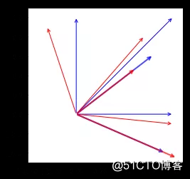
特征值和特征向量

A = np.array([[1, -0.3], [-0.1, 0.9]])
evalues, evectors = linalg.eig(A)

print(evalues)
print(evectors)

[1.13027756+0.j 0.76972244+0.j]
[[ 0.91724574 0.79325185]
[-0.3983218 0.60889368]]

#%figonly=线性变换将蓝色箭头变换为红色箭头
points = np.array([[0, 1.0], [1.0, 0], [1, 1]])

def draw_arrows(points, **kw):
props = dict(color="blue", arrowstyle="->")
props.update(kw)
for x, y in points:
pl.annotate("",
xy=(x, y), xycoords='data',
xytext=(0, 0), textcoords='data',
arrowprops=props)

draw_arrows(points)
draw_arrows(np.dot(A, points.T).T, color="red")
draw_arrows(evectors.T, alpha=0.7, linewidth=2)
draw_arrows(np.dot(A, evectors).T, color="red", alpha=0.7, linewidth=2)

ax = pl.gca()
ax.set_aspect("equal")
ax.set_xlim(-0.5, 1.1)
ax.set_ylim(-0.5, 1.1);

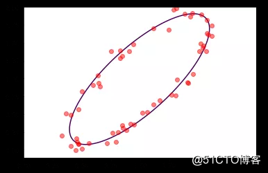
np.random.seed(42)
t = np.random.uniform(0, 2*np.pi, 60)

alpha = 0.4
a = 0.5
b = 1.0
x = 1.0 + a*np.cos(t)*np.cos(alpha) - b*np.sin(t)*np.sin(alpha)
y = 1.0 + a*np.cos(t)*np.sin(alpha) - b*np.sin(t)*np.cos(alpha)
x += np.random.normal(0, 0.05, size=len(x))
y += np.random.normal(0, 0.05, size=len(y))

D = np.c_[x**2, x*y, y**2, x, y, np.ones_like(x)]
A = np.dot(D.T, D)
C = np.zeros((6, 6))
C[[0, 1, 2], [2, 1, 0]] = 2, -1, 2
evalues, evectors = linalg.eig(A, C)     #❶
evectors = np.real(evectors)
err = np.mean(np.dot(D, evectors)**2, 0) #❷
p = evectors[:, np.argmin(err) ]         #❸
print (p)

[-0.55214278 0.5580915 -0.23809922 0.54584559 -0.08350449 -0.14852803]

#%figonly=用广义特征向量计算的拟合椭圆
def ellipse(p, x, y):
a, b, c, d, e, f = p
return a*x**2 + b*x*y + c*y**2 + d*x + e*y + f

X, Y = np.mgrid[0:2:100j, 0:2:100j]
Z = ellipse(p, X, Y)
pl.plot(x, y, "ro", alpha=0.5)
pl.contour(X, Y, Z, levels=[0]);

奇异值分解-SVD

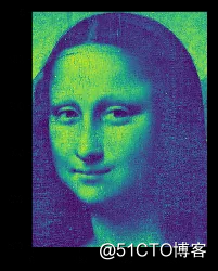
r, g, b = np.rollaxis(pl.imread("vinci_target.png"), 2).astype(float)
img = 0.2989 * r + 0.5870 * g + 0.1140 * b
img.shape

(505, 375)

U, s, Vh = linalg.svd(img)
print(U.shape)
print(s.shape)
print(Vh.shape)

(505, 505)
(375,)
(375, 375)

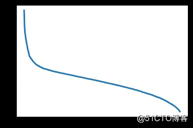
#%fig=按从大到小排列的奇异值
pl.semilogy(s, lw=3);

output_20_1

def composite(U, s, Vh, n):
return np.dot(U[:, :n], s[:n, np.newaxis] * Vh[:n, :])

print (np.allclose(img, composite(U, s, Vh, len(s))))

True

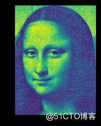
#%fig=原始图像、使用10、20、50个向量合成的图像（从左到右）
img10 = composite(U, s, Vh, 10)
img20 = composite(U, s, Vh, 20)
img50 = composite(U, s, Vh, 50)

%array_image img; img10; img20; img50

UsageError: Line magic function

%array_image

not found.

pl.imshow(img)

pl.imshow(img10)

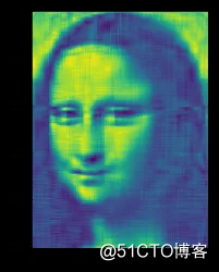
pl.imshow(img20)

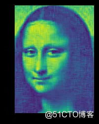
pl.imshow(img50)

4.统计-stats

import numpy as np
import pylab as pl
from scipy import stats

import matplotlib.pyplot as plt
import matplotlib as mpl
mpl.rcParams['font.sans-serif'] = ['SimHei']

连续概率分布

from scipy import stats
[k for k, v in stats.__dict__.items() if isinstance(v, stats.rv_continuous)]

['ksone',
'kstwobign',
'norm',
'alpha',
'anglit',
'arcsine',
'beta',
'betaprime',
'bradford',
'burr',
'burr12',
'fisk',
'cauchy',
'chi',
'chi2',
'cosine',
'dgamma',
'dweibull',
'expon',
'exponnorm',
'exponweib',
'exponpow',
'fatiguelife',
'foldcauchy',
'f',
'foldnorm',
'weibull_min',
'weibull_max',
'frechet_r',
'frechet_l',
'genlogistic',
'genpareto',
'genexpon',
'genextreme',
'gamma',
'erlang',
'gengamma',
'genhalflogistic',
'gompertz',
'gumbel_r',
'gumbel_l',
'halfcauchy',
'halflogistic',
'halfnorm',
'hypsecant',
'gausshyper',
'invgamma',
'invgauss',
'invweibull',
'johnsonsb',
'johnsonsu',
'laplace',
'levy',
'levy_l',
'levy_stable',
'logistic',
'loggamma',
'loglaplace',
'lognorm',
'gilbrat',
'maxwell',
'mielke',
'kappa4',
'kappa3',
'nakagami',
'ncx2',
'ncf',
't',
'nct',
'pareto',
'lomax',
'pearson3',
'powerlaw',
'powerlognorm',
'powernorm',
'rdist',
'rayleigh',
'reciprocal',
'rice',
'recipinvgauss',
'semicircular',
'skewnorm',
'trapz',
'triang',
'truncexpon',
'truncnorm',
'tukeylambda',
'uniform',
'vonmises',
'vonmises_line',
'wald',
'wrapcauchy',
'gennorm',
'halfgennorm',
'crystalball',
'argus']

stats.norm.stats()

(array(0.), array(1.))

X = stats.norm(loc=1.0, scale=2.0)
X.stats()

(array(1.), array(4.))

x = X.rvs(size=10000) # 对随机变量取10000个值
np.mean(x), np.var(x) # 期望值和方差

(1.0048352738823323, 3.9372117720073554)

stats.norm.fit(x) # 得到随机序列期望值和标准差

(1.0048352738823323, 1.984240855341749)

pdf, t = np.histogram(x, bins=100, normed=True)  #❶
t = (t[:-1] + t[1:]) * 0.5  #❷
cdf = np.cumsum(pdf) * (t[1] - t[0])  #❸
p_error = pdf - X.pdf(t)
c_error = cdf - X.cdf(t)
print ("max pdf error: {}, max cdf error: {}".format(
np.abs(p_error).max(),
np.abs(c_error).max()))

max pdf error: 0.018998755595167102, max cdf error: 0.018503342378306975

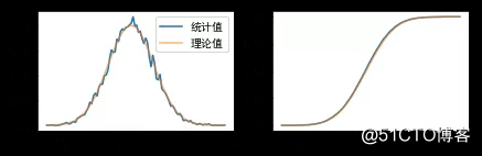
#%figonly=正态分布的概率密度函数（左）和累积分布函数（右）
fig, (ax1, ax2) = pl.subplots(1, 2, figsize=(7, 2))
ax1.plot(t, pdf, label=u"统计值")
ax1.plot(t, X.pdf(t), label=u"理论值", alpha=0.6)
ax1.legend(loc="best")
ax2.plot(t, cdf)
ax2.plot(t, X.cdf(t), alpha=0.6);

print(stats.gamma.stats(1.0))
print(stats.gamma.stats(2.0))

(array(1.), array(1.))
(array(2.), array(2.))

stats.gamma.stats(2.0, scale=2)

(array(4.), array(8.))

x = stats.gamma.rvs(2, scale=2, size=4)
x

array([4.40563983, 6.17699951, 3.65503843, 3.28052152])

stats.gamma.pdf(x, 2, scale=2)

array([0.12169605, 0.07037188, 0.14694352, 0.15904745])

X = stats.gamma(2, scale=2)
X.pdf(x)

array([0.12169605, 0.07037188, 0.14694352, 0.15904745])

离散概率分布

x = range(1, 7)
p = (0.4, 0.2, 0.1, 0.1, 0.1, 0.1)

dice = stats.rv_discrete(values=(x, p))
dice.rvs(size=20)

array([2, 5, 2, 6, 1, 6, 6, 5, 3, 1, 5, 2, 1, 1, 1, 1, 1, 2, 1, 6])

np.random.seed(42)
samples = dice.rvs(size=(20000, 50))
samples_mean = np.mean(samples, axis=1)

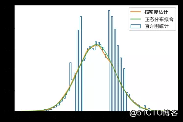
核密度估计

#%fig=核密度估计能更准确地表示随机变量的概率密度函数
_, bins, step = pl.hist(
samples_mean, bins=100, normed=True, histtype="step", label=u"直方图统计")
kde = stats.kde.gaussian_kde(samples_mean)
x = np.linspace(bins[0], bins[-1], 100)
pl.plot(x, kde(x), label=u"核密度估计")
mean, std = stats.norm.fit(samples_mean)
pl.plot(x, stats.norm(mean, std).pdf(x), alpha=0.8, label=u"正态分布拟合")
pl.legend()

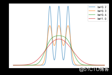
#%fig=`bw_method`参数越大核密度估计曲线越平滑
for bw in [0.2, 0.3, 0.6, 1.0]:
kde = stats.gaussian_kde([-1, 0, 1], bw_method=bw)
x = np.linspace(-5, 5, 1000)
y = kde(x)
pl.plot(x, y, lw=2, label="bw={}".format(bw), alpha=0.6)
pl.legend(loc="best");

二项、泊松、伽玛分布

stats.binom.pmf(range(6), 5, 1/6.0)

array([4.01877572e-01, 4.01877572e-01, 1.60751029e-01, 3.21502058e-02,
3.21502058e-03, 1.28600823e-04])

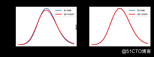
#%fig=当n足够大时二项分布和泊松分布近似相等
lambda_ = 10.0
x = np.arange(20)

n1, n2 = 100, 1000

y_binom_n1 = stats.binom.pmf(x, n1, lambda_ / n1)
y_binom_n2 = stats.binom.pmf(x, n2, lambda_ / n2)
y_poisson = stats.poisson.pmf(x, lambda_)
print(np.max(np.abs(y_binom_n1 - y_poisson)))
print(np.max(np.abs(y_binom_n2 - y_poisson)))
#%hide
fig, (ax1, ax2) = pl.subplots(1, 2, figsize=(7.5, 2.5))

ax1.plot(x, y_binom_n1, label=u"binom", lw=2)
ax1.plot(x, y_poisson, label=u"poisson", lw=2, color="red")
ax2.plot(x, y_binom_n2, label=u"binom", lw=2)
ax2.plot(x, y_poisson, label=u"poisson", lw=2, color="red")
for n, ax in zip((n1, n2), (ax1, ax2)):
ax.set_xlabel(u"次数")
ax.set_ylabel(u"概率")
ax.set_title("n={}".format(n))
ax.legend()
fig.subplots_adjust(0.1, 0.15, 0.95, 0.90, 0.2, 0.1)

0.00675531110335309
0.0006301754049777564

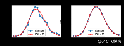
#%fig=模拟泊松分布
np.random.seed(42)
def sim_poisson(lambda_, time):
t = np.random.uniform(0, time, size=lambda_ * time)  #❶
count, time_edges = np.histogram(t, bins=time, range=(0, time))  #❷
dist, count_edges = np.histogram(
count, bins=20, range=(0, 20), density=True)  #❸
x = count_edges[:-1]
poisson = stats.poisson.pmf(x, lambda_)
return x, poisson, dist

lambda_ = 10
times = 1000, 50000
x1, poisson1, dist1 = sim_poisson(lambda_, times[0])
x2, poisson2, dist2 = sim_poisson(lambda_, times[1])
max_error1 = np.max(np.abs(dist1 - poisson1))
max_error2 = np.max(np.abs(dist2 - poisson2))
print("time={}, max_error={}".format(times[0], max_error1))
print("time={}, max_error={}".format(times[1], max_error2))
#%hide
fig, (ax1, ax2) = pl.subplots(1, 2, figsize=(7.5, 2.5))

ax1.plot(x1, dist1, "-o", lw=2, label=u"统计结果")
ax1.plot(x1, poisson1, "->", lw=2, label=u"泊松分布", color="red", alpha=0.6)
ax2.plot(x2, dist2, "-o", lw=2, label=u"统计结果")
ax2.plot(x2, poisson2, "->", lw=2, label=u"泊松分布", color="red", alpha=0.6)

for ax, time in zip((ax1, ax2), times):
ax.set_xlabel(u"次数")
ax.set_ylabel(u"概率")
ax.set_title(u"time = {}".format(time))
ax.legend(loc="lower center")

fig.subplots_adjust(0.1, 0.15, 0.95, 0.90, 0.2, 0.1)

time=1000, max_error=0.01964230201602718
time=50000, max_error=0.001798012894964722

#%fig=模拟伽玛分布
def sim_gamma(lambda_, time, k):
t = np.random.uniform(0, time, size=lambda_ * time) #❶
t.sort()  #❷
interval = t[k:] - t[:-k] #❸
dist, interval_edges = np.histogram(interval, bins=100, density=True) #❹
x = (interval_edges[1:] + interval_edges[:-1])/2  #❺
gamma = stats.gamma.pdf(x, k, scale=1.0/lambda_) #❺
return x, gamma, dist

lambda_ = 10
time = 1000
ks = 1, 2
x1, gamma1, dist1 = sim_gamma(lambda_, time, ks[0])
x2, gamma2, dist2 = sim_gamma(lambda_, time, ks[1])
#%hide
fig, (ax1, ax2) = pl.subplots(1, 2, figsize=(7.5, 2.5))

ax1.plot(x1, dist1,  lw=2, label=u"统计结果")
ax1.plot(x1, gamma1, lw=2, label=u"伽玛分布", color="red", alpha=0.6)
ax2.plot(x2, dist2,  lw=2, label=u"统计结果")
ax2.plot(x2, gamma2, lw=2, label=u"伽玛分布", color="red", alpha=0.6)

for ax, k in zip((ax1, ax2), ks):
ax.set_xlabel(u"时间间隔")
ax.set_ylabel(u"概率密度")
ax.set_title(u"k = {}".format(k))
ax.legend(loc="upper right")

fig.subplots_adjust(0.1, 0.15, 0.95, 0.90, 0.2, 0.1);

png

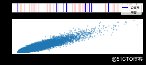
T = 100000
A_count = int(T / 5)
B_count = int(T / 10)

A_time = np.random.uniform(0, T, A_count) #❶
B_time = np.random.uniform(0, T, B_count)

bus_time = np.concatenate((A_time, B_time)) #❷
bus_time.sort()

N = 200000
passenger_time = np.random.uniform(bus_time[0], bus_time[-1], N) #❸

idx = np.searchsorted(bus_time, passenger_time) #❹
np.mean(bus_time[idx] - passenger_time) * 60    #❺

202.3388747879705

np.mean(np.diff(bus_time)) * 60

199.99833251643057

#%figonly=观察者偏差
import matplotlib.gridspec as gridspec
pl.figure(figsize=(7.5, 3))

G = gridspec.GridSpec(10, 1)
ax1 = pl.subplot(G[:2,  0])
ax2 = pl.subplot(G[3:, 0])

ax1.vlines(bus_time[:10], 0, 1, lw=2, color="blue", label=u"公交车")
ptime = np.random.uniform(bus_time[0], bus_time[9], 100)
ax1.vlines(ptime, 0, 1, lw=1, color="red", alpha=0.2, label=u"乘客")
ax1.legend()
count, bins = np.histogram(passenger_time, bins=bus_time)
ax2.plot(np.diff(bins), count, ".", alpha=0.3, rasterized=True)
ax2.set_xlabel(u"公交车的时间间隔")
ax2.set_ylabel(u"等待人数");

from scipy import integrate
t = 10.0 / 3  # 两辆公交车之间的平均时间间隔
bus_interval = stats.gamma(1, scale=t)
n, _ = integrate.quad(lambda x: 0.5 * x * x * bus_interval.pdf(x), 0, 1000)
d, _ = integrate.quad(lambda x: x * bus_interval.pdf(x), 0, 1000)
n / d * 60

200.0

学生 t-分布与 t 检验

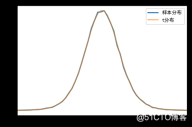
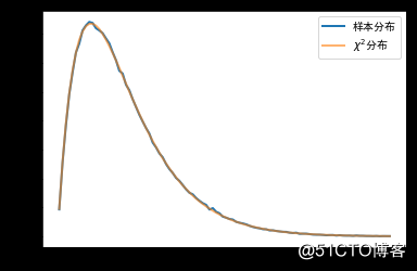
#%fig=模拟学生t-分布
mu = 0.0
n = 10
samples = stats.norm(mu).rvs(size=(100000, n))  #❶
t_samples = (np.mean(samples, axis=1) - mu) / np.std(
samples, ddof=1, axis=1) * n**0.5  #❷
sample_dist, x = np.histogram(t_samples, bins=100, density=True)  #❸
x = 0.5 * (x[:-1] + x[1:])
t_dist = stats.t(n - 1).pdf(x)
print("max error:", np.max(np.abs(sample_dist - t_dist)))
#%hide
pl.plot(x, sample_dist, lw=2, label=u"样本分布")
pl.plot(x, t_dist, lw=2, alpha=0.6, label=u"t分布")
pl.xlim(-5, 5)
pl.legend(loc="best")

max error: 0.006832108369761447

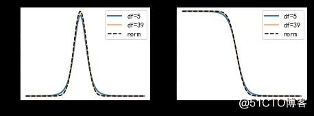
#%figonly=当`df`增大，学生t-分布趋向于正态分布
fig, (ax1, ax2) = pl.subplots(1, 2, figsize=(7.5, 2.5))
ax1.plot(x, stats.t(6-1).pdf(x), label=u"df=5", lw=2)
ax1.plot(x, stats.t(40-1).pdf(x), label=u"df=39", lw=2, alpha=0.6)
ax1.plot(x, stats.norm.pdf(x), "k--", label=u"norm")
ax1.legend()

ax2.plot(x, stats.t(6-1).sf(x), label=u"df=5", lw=2)
ax2.plot(x, stats.t(40-1).sf(x), label=u"df=39", lw=2, alpha=0.6)
ax2.plot(x, stats.norm.sf(x), "k--", label=u"norm")
ax2.legend();

n = 30
np.random.seed(42)
s = stats.norm.rvs(loc=1, scale=0.8, size=n)

t = (np.mean(s) - 0.5) / (np.std(s, ddof=1) / np.sqrt(n))
print (t, stats.ttest_1samp(s, 0.5))

2.658584340882224
Ttest_1sampResult(statistic=2.658584340882224, pvalue=0.01263770225709123)

print ((np.mean(s) - 1) / (np.std(s, ddof=1) / np.sqrt(n)))
print (stats.ttest_1samp(s, 1), stats.ttest_1samp(s, 0.9))

-1.1450173670383303
Ttest_1sampResult(statistic=-1.1450173670383303, pvalue=0.26156414618801477) Ttest_1sampResult(statistic=-0.3842970254542196, pvalue=0.7035619103425202)

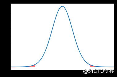
#%fig=红色部分为`ttest_1samp()`计算的p值
x = np.linspace(-5, 5, 500)
y = stats.t(n-1).pdf(x)
plt.plot(x, y, lw=2)
t, p = stats.ttest_1samp(s, 0.5)
mask = x > np.abs(t)
plt.fill_between(x[mask], y[mask], color="red", alpha=0.5)
mask = x < -np.abs(t)
plt.fill_between(x[mask], y[mask], color="red", alpha=0.5)
plt.axhline(color="k", lw=0.5)
plt.xlim(-5, 5);

from scipy import integrate
x = np.linspace(-10, 10, 100000)
y = stats.t(n-1).pdf(x)
mask = x >= np.abs(t)
integrate.trapz(y[mask], x[mask])*2

0.012633433707685974

m = 200000
mean = 0.5
r = stats.norm.rvs(loc=mean, scale=0.8, size=(m, n))
ts = (np.mean(s) - mean) / (np.std(s, ddof=1) / np.sqrt(n))
tr = (np.mean(r, axis=1) - mean) / (np.std(r, ddof=1, axis=1) / np.sqrt(n))
np.mean(np.abs(tr) > np.abs(ts))

0.012695

np.random.seed(42)

s1 = stats.norm.rvs(loc=1, scale=1.0, size=20)
s2 = stats.norm.rvs(loc=1.5, scale=0.5, size=20)
s3 = stats.norm.rvs(loc=1.5, scale=0.5, size=25)

print (stats.ttest_ind(s1, s2, equal_var=False)) #❶
print (stats.ttest_ind(s2, s3, equal_var=True))  #❷

Ttest_indResult(statistic=-2.2391470627176755, pvalue=0.033250866086743665)
Ttest_indResult(statistic=-0.5946698521856172, pvalue=0.5551805875810539)

卡方分布和卡方检验

#%fig=使用随机数验证卡方分布
a = np.random.normal(size=(300000, 4))
cs = np.sum(a**2, axis=1)

sample_dist, bins = np.histogram(cs, bins=100, range=(0, 20), density=True)
x = 0.5 * (bins[:-1] + bins[1:])
chi2_dist = stats.chi2.pdf(x, 4)
print("max error:", np.max(np.abs(sample_dist - chi2_dist)))
#%hide
pl.plot(x, sample_dist, lw=2, label=u"样本分布")
pl.plot(x, chi2_dist, lw=2, alpha=0.6, label=u"$\chi ^{2}$分布")
pl.legend(loc="best")

max error: 0.0030732520533635066

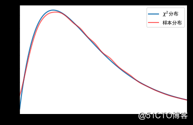
#%fig=模拟卡方分布
repeat_count = 60000
n, k = 100, 5

np.random.seed(42)
ball_ids = np.random.randint(0, k, size=(repeat_count, n)) #❶
counts = np.apply_along_axis(np.bincount, 1, ball_ids, minlength=k) #❷
cs2 = np.sum((counts - n/k)**2.0/(n/k), axis=1) #❸
k = stats.kde.gaussian_kde(cs2) #❹
x = np.linspace(0, 10, 200)
pl.plot(x, stats.chi2.pdf(x, 4), lw=2, label=u"$\chi ^{2}$分布")
pl.plot(x, k(x), lw=2, color="red", alpha=0.6, label=u"样本分布")
pl.legend(loc="best")
pl.xlim(0, 10);

def choose_balls(probabilities, size):
r = stats.rv_discrete(values=(range(len(probabilities)), probabilities))
s = r.rvs(size=size)
counts = np.bincount(s)
return counts

np.random.seed(42)
counts1 = choose_balls([0.18, 0.24, 0.25, 0.16, 0.17], 400)
counts2 = choose_balls([0.2]*5, 400)

print(counts1)
print(counts2)

[80 93 97 64 66]
[89 76 79 71 85]

chi1, p1 = stats.chisquare(counts1)
chi2, p2 = stats.chisquare(counts2)

print ("chi1 =", chi1, "p1 =", p1)
print ("chi2 =", chi2, "p2 =", p2)

chi1 = 11.375 p1 = 0.022657601239769634
chi2 = 2.55 p2 = 0.6357054527037017

#%figonly=卡方检验计算的概率为阴影部分的面积
x = np.linspace(0, 30, 200)
CHI2 = stats.chi2(4)
pl.plot(x, CHI2.pdf(x), "k", lw=2)
pl.vlines(chi1, 0, CHI2.pdf(chi1))
pl.vlines(chi2, 0, CHI2.pdf(chi2))
pl.fill_between(x[x>chi1], 0, CHI2.pdf(x[x>chi1]), color="red", alpha=1.0)
pl.fill_between(x[x>chi2], 0, CHI2.pdf(x[x>chi2]), color="green", alpha=0.5)
pl.text(chi1, 0.015, r"$\chi^2_1$", fontsize=14)
pl.text(chi2, 0.015, r"$\chi^2_2$", fontsize=14)
pl.ylim(0, 0.2)
pl.xlim(0, 20);

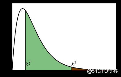
table = [[43, 9], [44, 4]]
chi2, p, dof, expected = stats.chi2_contingency(table)
print(chi2)
print(p)

1.0724852071005921
0.300384770390566

stats.fisher_exact(table)

(0.43434343434343436, 0.23915695682224306)

5.数值积分-integrate

import pylab as pl
import numpy as np
from scipy import integrate
from scipy.integrate import odeint
import matplotlib as mpl
mpl.rcParams['font.sans-serif'] = ['SimHei']

球的体积

def half_circle(x):
return (1-x**2)**0.5

N = 10000
x = np.linspace(-1, 1, N)
dx = x[1] - x[0]
y = half_circle(x)
2 * dx * np.sum(y) # 面积的两倍

3.1415893269307373

np.trapz(y, x) * 2 # 面积的两倍

3.1415893269315975

from scipy import integrate
pi_half, err = integrate.quad(half_circle, -1, 1)
pi_half * 2

3.141592653589797

def half_sphere(x, y):
return (1-x**2-y**2)**0.5

volume, error = integrate.dblquad(half_sphere, -1, 1,
lambda x:-half_circle(x),
lambda x:half_circle(x))

print (volume, error, np.pi*4/3/2)

2.094395102393199 1.0002356720661965e-09 2.0943951023931953

解常微分方程组

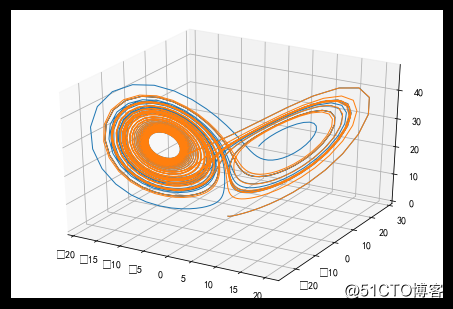
#%fig=洛伦茨吸引子：微小的初值差别也会显著地影响运动轨迹
from scipy.integrate import odeint
import numpy as np

def lorenz(w, t, p, r, b): #❶
# 给出位置矢量w，和三个参数p, r, b计算出
# dx/dt, dy/dt, dz/dt的值
x, y, z = w.tolist()
# 直接与lorenz的计算公式对应
return p*(y-x), x*(r-z)-y, x*y-b*z

t = np.arange(0, 30, 0.02) # 创建时间点
# 调用ode对lorenz进行求解, 用两个不同的初始值
track1 = odeint(lorenz, (0.0, 1.00, 0.0), t, args=(10.0, 28.0, 3.0)) #❷
track2 = odeint(lorenz, (0.0, 1.01, 0.0), t, args=(10.0, 28.0, 3.0)) #❸
#%hide
from mpl_toolkits.mplot3d import Axes3D
fig = pl.figure()
ax = Axes3D(fig)
ax.plot(track1[:,0], track1[:,1], track1[:,2], lw=1)
ax.plot(track2[:,0], track2[:,1], track2[:,2], lw=1);

ode 类

def mass_spring_damper(xu, t, m, k, b, F):
x, u = xu.tolist()
dx = u
du = (F - k*x - b*u)/m
return dx, du

#%fig=滑块的速度和位移曲线
m, b, k, F = 1.0, 10.0, 20.0, 1.0
init_status = 0.0, 0.0
args = m, k, b, F
t = np.arange(0, 2, 0.01)
result = odeint(mass_spring_damper, init_status, t, args)
#%hide
fig, (ax1, ax2) = pl.subplots(2, 1)
ax1.plot(t, result[:, 0], label=u"位移")
ax1.legend()
ax2.plot(t, result[:, 1], label=u"速度")
ax2.legend();

from scipy.integrate import ode

class MassSpringDamper(object): #❶

def __init__(self, m, k, b, F):
self.m, self.k, self.b, self.F = m, k, b, F

def f(self, t, xu):
x, u = xu.tolist()
dx = u
du = (self.F - self.k*x - self.b*u)/self.m
return [dx, du]

system = MassSpringDamper(m=m, k=k, b=b, F=F)
init_status = 0.0, 0.0
dt = 0.01

r = ode(system.f) #❷
r.set_integrator('vode', method='bdf')
r.set_initial_value(init_status, 0)

t = []
result2 = [init_status]
while r.successful() and r.t + dt < 2: #❸
r.integrate(r.t + dt)
t.append(r.t)
result2.append(r.y)

result2 = np.array(result2)
np.allclose(result, result2)

True

class PID(object):

def __init__(self, kp, ki, kd, dt):
self.kp, self.ki, self.kd, self.dt = kp, ki, kd, dt
self.last_error = None
self.status = 0.0

def update(self, error):
p = self.kp * error
i = self.ki * self.status
if self.last_error is None:
d = 0.0
else:
d = self.kd * (error - self.last_error) / self.dt
self.status += error * self.dt
self.last_error = error
return p + i + d

#%fig=使用PID控制器让滑块停在位移为1.0处
def pid_control_system(kp, ki, kd, dt, target=1.0):
system = MassSpringDamper(m=m, k=k, b=b, F=0.0)
pid = PID(kp, ki, kd, dt)
init_status = 0.0, 0.0

r = ode(system.f)
r.set_integrator('vode', method='bdf')
r.set_initial_value(init_status, 0)

t = [0]
result = [init_status]
F_arr = [0]

while r.successful() and r.t + dt < 2.0:
r.integrate(r.t + dt)
err = target - r.y[0]  #❶
F = pid.update(err)  #❷
system.F = F  #❸
t.append(r.t)
result.append(r.y)
F_arr.append(F)

result = np.array(result)
t = np.array(t)
F_arr = np.array(F_arr)
return t, F_arr, result

t, F_arr, result = pid_control_system(50.0, 100.0, 10.0, 0.001)
print(u"控制力的终值:", F_arr[-1])
#%hide
fig, (ax1, ax2, ax3) = pl.subplots(3, 1, figsize=(6, 6))
ax1.plot(t, result[:, 0], label=u"位移")
ax1.legend(loc="best")
ax2.plot(t, result[:, 1], label=u"速度")
ax2.legend(loc="best")
ax3.plot(t, F_arr, label=u"控制力")
ax3.legend(loc="best")

控制力的终值: 19.943404699515057

%%time
from scipy import optimize

def eval_func(k):
kp, ki, kd = k
t, F_arr, result = pid_control_system(kp, ki, kd, 0.01)
return np.sum(np.abs(result[:, 0] - 1.0))

kwargs = {
"method": "L-BFGS-B",
"bounds": [(10, 200), (10, 100), (1, 100)],
"options": {
"approx_grad": True
}
}

opt_k = optimize.basinhopping(
eval_func, (10, 10, 10), niter=10, minimizer_kwargs=kwargs)
print(opt_k.x)

[56.67106149 99.97434757 1.33963577]
Wall time: 55.1 s

#%fig=优化PID的参数降低控制响应时间
kp, ki, kd = opt_k.x
t, F_arr, result = pid_control_system(kp, ki, kd, 0.01)
idx = np.argmin(np.abs(t - 0.5))
x, u = result[idx]
print ("t={}, x={:g}, u={:g}".format(t[idx], x, u))
#%hide
fig, (ax1, ax2, ax3) = pl.subplots(3, 1, figsize=(6, 6))
ax1.plot(t, result[:, 0], label=u"位移")
ax1.legend(loc="best")
ax2.plot(t, result[:, 1], label=u"速度")
ax2.legend(loc="best")
ax3.plot(t, F_arr, label=u"控制力")
ax3.legend(loc="best");

t=0.5000000000000002, x=1.07098, u=0.315352

6.信号处理-signal

import pylab as pl
import numpy as np
from scipy import signal

import matplotlib as mpl
mpl.rcParams['font.sans-serif'] = ['SimHei']

中值滤波

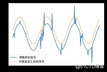
#%fig=使用中值滤波剔除瞬间噪声
t = np.arange(0, 20, 0.1)
x = np.sin(t)
x[np.random.randint(0, len(t), 20)] += np.random.standard_normal(20)*0.6 #❶
x2 = signal.medfilt(x, 5) #❷
x3 = signal.order_filter(x, np.ones(5), 2)
print (np.all(x2 == x3))
pl.plot(t, x, label=u"带噪声的信号")
pl.plot(t, x2 + 0.5, alpha=0.6, label=u"中值滤波之后的信号")
pl.legend(loc="best");

True

output_4_1

滤波器设计

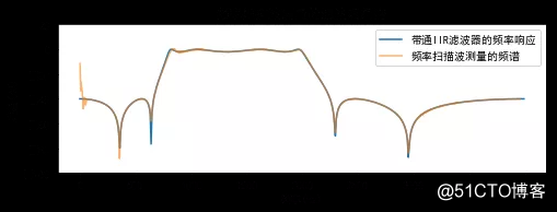
sampling_rate = 8000.0

# 设计一个带通滤波器：
# 通带为0.2*4000 - 0.5*4000
# 阻带为<0.1*4000, >0.6*4000
# 通带增益的最大衰减值为2dB
# 阻带的最小衰减值为40dB
b, a = signal.iirdesign([0.2, 0.5], [0.1, 0.6], 2, 40) #❶

# 使用freq计算滤波器的频率响应
w, h = signal.freqz(b, a) #❷

# 计算增益
power = 20*np.log10(np.clip(np.abs(h), 1e-8, 1e100)) #❸
freq = w / np.pi * sampling_rate / 2

#%fig=用频率扫描波测量的频率响应
# 产生2秒钟的取样频率为sampling_rate Hz的频率扫描信号
# 开始频率为0， 结束频率为sampling_rate/2
t = np.arange(0, 2, 1/sampling_rate) #❶
sweep = signal.chirp(t, f0=0, t1=2, f1=sampling_rate/2) #❷
# 对频率扫描信号进行滤波
out = signal.lfilter(b, a, sweep) #❸
# 将波形转换为能量
out = 20*np.log10(np.abs(out)) #❹
# 找到所有局部最大值的下标
index = signal.argrelmax(out, order=3)  #❺
# 绘制滤波之后的波形的增益
pl.figure(figsize=(8, 2.5))
pl.plot(freq, power, label=u"带通IIR滤波器的频率响应")
pl.plot(t[index]/2.0*4000, out[index], label=u"频率扫描波测量的频谱", alpha=0.6) #❻
pl.legend(loc="best")
#%hide
pl.title(u"频率扫描波测量的滤波器频谱")
pl.ylim(-100,20)
pl.ylabel(u"增益(dB)")
pl.xlabel(u"频率(Hz)");

连续时间线性系统

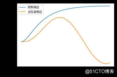
#%fig=系统的阶跃响应和正弦波响应
m, b, k = 1.0, 10, 20

numerator = [1]
denominator = [m, b, k]

plant = signal.lti(numerator, denominator)  #❶

t = np.arange(0, 2, 0.01)
_, x_step = plant.step(T=t)  #❷
_, x_sin, _ = signal.lsim(plant, U=np.sin(np.pi * t), T=t)  #❸
#%hide
pl.plot(t, x_step, label=u"阶跃响应")
pl.plot(t, x_sin, label=u"正弦波响应")
pl.legend(loc="best")
pl.xlabel(u"时间（秒）")
pl.ylabel(u"位移（米）")

Text(0,0.5,'位移（米）')

7.插值-interpolate

import numpy as np
import pylab as pl
from scipy import interpolate

import matplotlib as mpl
mpl.rcParams['font.sans-serif'] = ['SimHei']

一维插值

WARNING：高次interp1d()插值的运算量很大，因此对于点数较多的数据，建议使用后面介绍的UnivariateSpline()。

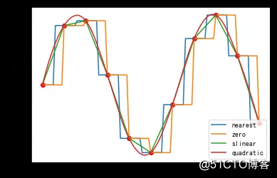
#%fig=`interp1d`的各阶插值
from scipy import interpolate

x = np.linspace(0, 10, 11)
y = np.sin(x)

xnew = np.linspace(0, 10, 101)
pl.plot(x, y, 'ro')
for kind in ['nearest', 'zero', 'slinear', 'quadratic']:
f = interpolate.interp1d(x, y, kind=kind)  #❶
ynew = f(xnew)  #❷
pl.plot(xnew, ynew, label=str(kind))

pl.legend(loc='lower right')

output_5_1

外推和 Spline 拟合

#%fig=使用UnivariateSpline进行插值：外推（上），数据拟合（下）
x1 = np.linspace(0, 10, 20)
y1 = np.sin(x1)
sx1 = np.linspace(0, 12, 100)
sy1 = interpolate.UnivariateSpline(x1, y1, s=0)(sx1)  #❶

x2 = np.linspace(0, 20, 200)
y2 = np.sin(x2) + np.random.standard_normal(len(x2)) * 0.2
sx2 = np.linspace(0, 20, 2000)
spline2 = interpolate.UnivariateSpline(x2, y2, s=8)  #❷
sy2 = spline2(sx2)

pl.figure(figsize=(8, 5))
pl.subplot(211)
pl.plot(x1, y1, ".", label=u"数据点")
pl.plot(sx1, sy1, label=u"spline曲线")
pl.legend()

pl.subplot(212)
pl.plot(x2, y2, ".", label=u"数据点")
pl.plot(sx2, sy2, linewidth=2, label=u"spline曲线")
pl.plot(x2, np.sin(x2), label=u"无噪声曲线")
pl.legend()

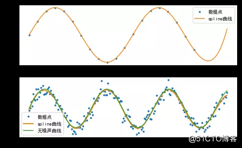
output_7_1

print(np.array_str(spline2.roots(), precision=3))

[ 0.053 3.151 6.36 9.386 12.603 15.619 18.929]

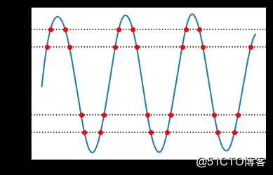
#%fig=计算Spline与水平线的交点
def roots_at(self, v):  #❶
coeff = self.get_coeffs()
coeff -= v
try:
root = self.roots()
return root
finally:
coeff += v

interpolate.UnivariateSpline.roots_at = roots_at  #❷

pl.plot(sx2, sy2, linewidth=2, label=u"spline曲线")

ax = pl.gca()
for level in [0.5, 0.75, -0.5, -0.75]:
ax.axhline(level, ls=":", color="k")
xr = spline2.roots_at(level)  #❸
pl.plot(xr, spline2(xr), "ro")

参数插值

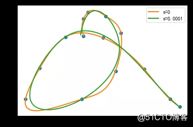
#%fig=使用参数插值连接二维平面上的点
x = [
4.913, 4.913, 4.918, 4.938, 4.955, 4.949, 4.911, 4.848, 4.864, 4.893,
4.935, 4.981, 5.01, 5.021
]

y = [
5.2785, 5.2875, 5.291, 5.289, 5.28, 5.26, 5.245, 5.245, 5.2615, 5.278,
5.2775, 5.261, 5.245, 5.241
]

pl.plot(x, y, "o")

for s in (0, 1e-4):
tck, t = interpolate.splprep([x, y], s=s)  #❶
xi, yi = interpolate.splev(np.linspace(t[0], t[-1], 200), tck)  #❷
pl.plot(xi, yi, lw=2, label=u"s=%g" % s)

pl.legend()

单调插值

import numpy as np
import matplotlib.pyplot as plt
from scipy import interpolate

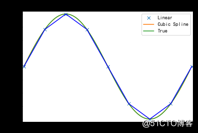
x = np.arange(0, 2 * np.pi + np.pi / 4, 2 * np.pi / 8)
y = np.sin(x)
tck = interpolate.splrep(x, y, s=0)
xnew = np.arange(0, 2 * np.pi, np.pi / 50)
ynew = interpolate.splev(xnew, tck, der=0)

plt.figure()
plt.plot(x, y, 'x', xnew, ynew, xnew, np.sin(xnew), x, y, 'b')
plt.legend(['Linear', 'Cubic Spline', 'True'])
plt.axis([-0.05, 6.33, -1.05, 1.05])
plt.title('三次样条插值')
plt.show()

多维插值

#%fig=使用interp2d类进行二维插值
def func(x, y):  #❶
return (x + y) * np.exp(-5.0 * (x**2 + y**2))

# X-Y轴分为15*15的网格
y, x = np.mgrid[-1:1:15j, -1:1:15j]  #❷
fvals = func(x, y)  # 计算每个网格点上的函数值

# 二维插值
newfunc = interpolate.interp2d(x, y, fvals, kind='cubic')  #❸

# 计算100*100的网格上的插值
xnew = np.linspace(-1, 1, 100)
ynew = np.linspace(-1, 1, 100)
fnew = newfunc(xnew, ynew)  #❹
#%hide
pl.subplot(121)
pl.imshow(
fvals,
extent=[-1, 1, -1, 1],
cmap=pl.cm.jet,
interpolation='nearest',
origin="lower")
pl.title("fvals")
pl.subplot(122)
pl.imshow(
fnew,
extent=[-1, 1, -1, 1],
cmap=pl.cm.jet,
interpolation='nearest',
origin="lower")
pl.title("fnew")
pl.show()

griddata

WARNING

griddata()使用欧几里得距离计算插值。如果 K 维空间中每个维度的取值范围相差较大，则应先将数据正规化，然后使用griddata()进行插值运算。

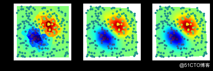
#%fig=使用gridata进行二维插值
# 计算随机N个点的坐标，以及这些点对应的函数值
N = 200
np.random.seed(42)
x = np.random.uniform(-1, 1, N)
y = np.random.uniform(-1, 1, N)
z = func(x, y)

yg, xg = np.mgrid[-1:1:100j, -1:1:100j]
xi = np.c_[xg.ravel(), yg.ravel()]

methods = 'nearest', 'linear', 'cubic'

zgs = [
interpolate.griddata((x, y), z, xi, method=method).reshape(100, 100)
for method in methods
]
#%hide
fig, axes = pl.subplots(1, 3, figsize=(11.5, 3.5))

for ax, method, zg in zip(axes, methods, zgs):
ax.imshow(
zg,
extent=[-1, 1, -1, 1],
cmap=pl.cm.jet,
interpolation='nearest',
origin="lower")
ax.set_xlabel(method)
ax.scatter(x, y, c=z)

径向基函数插值

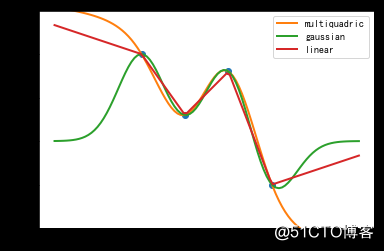
#%fig=一维RBF插值
from scipy.interpolate import Rbf

x1 = np.array([-1, 0, 2.0, 1.0])
y1 = np.array([1.0, 0.3, -0.5, 0.8])

funcs = ['multiquadric', 'gaussian', 'linear']
nx = np.linspace(-3, 4, 100)
rbfs = [Rbf(x1, y1, function=fname) for fname in funcs]  #❶
rbf_ys = [rbf(nx) for rbf in rbfs]  #❷
#%hide
pl.plot(x1, y1, "o")
for fname, ny in zip(funcs, rbf_ys):
pl.plot(nx, ny, label=fname, lw=2)

pl.ylim(-1.0, 1.5)
pl.legend()

output_20_1

for fname, rbf in zip(funcs, rbfs):
print (fname, rbf.nodes)

multiquadric [-0.88822885 2.17654513 1.42877511 -2.67919021]
gaussian [ 1.00321945 -0.02345964 -0.65441716 0.91375159]
linear [-0.26666667 0.6 0.73333333 -0.9 ]

#%fig=二维径向基函数插值
rbfs = [Rbf(x, y, z, function=fname) for fname in funcs]
rbf_zg = [rbf(xg, yg).reshape(xg.shape) for rbf in rbfs]
#%hide
fig, axes = pl.subplots(1, 3, figsize=(11.5, 3.5))
for ax, fname, zg in zip(axes, funcs, rbf_zg):
ax.imshow(
zg,
extent=[-1, 1, -1, 1],
cmap=pl.cm.jet,
interpolation='nearest',
origin="lower")
ax.set_xlabel(fname)
ax.scatter(x, y, c=z)

#%fig=`epsilon`参数指定径向基函数中数据点的作用范围
epsilons = 0.1, 0.15, 0.3
rbfs = [Rbf(x, y, z, function="gaussian", epsilon=eps) for eps in epsilons]
zgs = [rbf(xg, yg).reshape(xg.shape) for rbf in rbfs]
#%hide
fig, axes = pl.subplots(1, 3, figsize=(11.5, 3.5))
for ax, eps, zg in zip(axes, epsilons, zgs):
ax.imshow(
zg,
extent=[-1, 1, -1, 1],
cmap=pl.cm.jet,
interpolation='nearest',
origin="lower")
ax.set_xlabel("eps=%g" % eps)
ax.scatter(x, y, c=z)

8.稀疏矩阵-sparse

%matplotlib inline
import numpy as np
import pylab as pl
from scipy import sparse
from scipy.sparse import csgraph

稀疏矩阵的储存形式

from scipy import sparse
a = sparse.dok_matrix((10, 5))
a[2, 3] = 1.0
a[3, 3] = 2.0
a[4, 3] = 3.0
print(a.keys())
print(a.values())

dict_keys([(2, 3), (3, 3), (4, 3)])
dict_values([1.0, 2.0, 3.0])

b = sparse.lil_matrix((10, 5))
b[2, 3] = 1.0
b[3, 4] = 2.0
b[3, 2] = 3.0
print(b.data)
print(b.rows)

[list([]) list([]) list([1.0]) list([3.0, 2.0]) list([]) list([]) list([])
list([]) list([]) list([])]
[list([]) list([]) list([3]) list([2, 4]) list([]) list([]) list([])
list([]) list([]) list([])]

row = [2, 3, 3, 2]
col = [3, 4, 2, 3]
data = [1, 2, 3, 10]
c = sparse.coo_matrix((data, (row, col)), shape=(5, 6))
print (c.col, c.row, c.data)
print (c.toarray())

[3 4 2 3] [2 3 3 2] [ 1 2 3 10]
[[ 0 0 0 0 0 0]
[ 0 0 0 0 0 0]
[ 0 0 0 11 0 0]
[ 0 0 3 0 2 0]
[ 0 0 0 0 0 0]]

矩阵向量相乘

import numpy as np
from scipy.sparse import csr_matrix
A = csr_matrix([[1, 2, 0], [0, 0, 3], [4, 0, 5]])
v = np.array([1, 0, -1])
A.dot(v)

array([ 1, -3, -1], dtype=int32)

示例1

构造一个1000x1000 lil_matrix并添加值：

from scipy.sparse import lil_matrix
from scipy.sparse.linalg import spsolve
from numpy.linalg import solve, norm
from numpy.random import rand

A = lil_matrix((1000, 1000))
A[0, :100] = rand(100)
A[1, 100:200] = A[0, :100]
A.setdiag(rand(1000))

现在将其转换为CSR格式，并求解
的

：

A = A.tocsr()
b = rand(1000)
x = spsolve(A, b)

将其转换为密集矩阵并求解，并检查结果是否相同：

x_ = solve(A.toarray(), b)

现在我们可以使用以下公式计算错误的范数：

err = norm(x-x_)
err < 1e-10

True

示例2

构造COO格式的矩阵：

from scipy import sparse
from numpy import array
I = array([0,3,1,0])
J = array([0,3,1,2])
V = array([4,5,7,9])
A = sparse.coo_matrix((V,(I,J)),shape=(4,4))

注意，索引不需要排序。

转换为CSR或CSC时，将对重复的（i，j）条目进行求和。

I = array([0,0,1,3,1,0,0])
J = array([0,2,1,3,1,0,0])
V = array([1,1,1,1,1,1,1])
B = sparse.coo_matrix((V,(I,J)),shape=(4,4)).tocsr()

这对于构造有限元刚度矩阵和质量矩阵是有用的。

9.图像处理-ndimage

import numpy as np
import pylab as pl

形态学图像处理

import numpy as np

def expand_image(img, value, out=None, size = 10):
if out is None:
w, h = img.shape
out = np.zeros((w*size, h*size),dtype=np.uint8)

tmp = np.repeat(np.repeat(img,size,0),size,1)
out[:,:] = np.where(tmp, value, out)
out[::size,:] = 0
out[:,::size] = 0
return out

def show_image(*imgs):
for idx, img in enumerate(imgs, 1):
ax = pl.subplot(1, len(imgs), idx)
pl.imshow(img, cmap="gray")
ax.set_axis_off()
pl.subplots_adjust(0.02, 0, 0.98, 1, 0.02, 0)

膨胀和腐蚀

#%fig=四连通和八连通的膨胀运算
from scipy.ndimage import morphology

def dilation_demo(a, structure=None):
b = morphology.binary_dilation(a, structure)
img = expand_image(a, 255)
return expand_image(np.logical_xor(a,b), 150, out=img)

a = pl.imread("scipy_morphology_demo.png")[:,:,0].astype(np.uint8)
img1 = expand_image(a, 255)

img2 = dilation_demo(a)
img3 = dilation_demo(a, [[1,1,1],[1,1,1],[1,1,1]])
show_image(img1, img2, img3)

#%fig=不同结构元素的膨胀效果
img4 = dilation_demo(a, [[0,0,0],[1,1,1],[0,0,0]])
img5 = dilation_demo(a, [[0,1,0],[0,1,0],[0,1,0]])
img6 = dilation_demo(a, [[0,1,0],[0,1,0],[0,0,0]])
show_image(img4, img5, img6)

#%fig=四连通和八连通的腐蚀运算
def erosion_demo(a, structure=None):
b = morphology.binary_erosion(a, structure)
img = expand_image(a, 255)
return expand_image(np.logical_xor(a,b), 100, out=img)

img1 = expand_image(a, 255)
img2 = erosion_demo(a)
img3 = erosion_demo(a, [[1,1,1],[1,1,1],[1,1,1]])
show_image(img1, img2, img3)

Hit和Miss

#%fig=Hit和Miss运算
def hitmiss_demo(a, structure1, structure2):
b = morphology.binary_hit_or_miss(a, structure1, structure2)
img = expand_image(a, 100)
return expand_image(b, 255, out=img)

img1 = expand_image(a, 255)

img2 = hitmiss_demo(a, [[0,0,0],[0,1,0],[1,1,1]], [[1,0,0],[0,0,0],[0,0,0]])
img3 = hitmiss_demo(a, [[0,0,0],[0,0,0],[1,1,1]], [[1,0,0],[0,1,0],[0,0,0]])

show_image(img1, img2, img3)

#%fig=使用Hit和Miss进行细线化运算
def skeletonize(img):
h1 = np.array([[0, 0, 0],[0, 1, 0],[1, 1, 1]]) #❶
m1 = np.array([[1, 1, 1],[0, 0, 0],[0, 0, 0]])
h2 = np.array([[0, 0, 0],[1, 1, 0],[0, 1, 0]])
m2 = np.array([[0, 1, 1],[0, 0, 1],[0, 0, 0]])
hit_list = []
miss_list = []
for k in range(4): #❷
hit_list.append(np.rot90(h1, k))
hit_list.append(np.rot90(h2, k))
miss_list.append(np.rot90(m1, k))
miss_list.append(np.rot90(m2, k))
img = img.copy()
while True:
last = img
for hit, miss in zip(hit_list, miss_list):
hm = morphology.binary_hit_or_miss(img, hit, miss) #❸
# 从图像中删除hit_or_miss所得到的白色点
img = np.logical_and(img, np.logical_not(hm)) #❹
# 如果处理之后的图像和处理前的图像相同，则结束处理
if np.all(img == last): #❺
break
return img

a = pl.imread("scipy_morphology_demo2.png")[:,:,0].astype(np.uint8)
b = skeletonize(a)
#%hide
_, (ax1, ax2) = pl.subplots(1, 2, figsize=(9, 3))
ax1.imshow(a, cmap="gray", interpolation="nearest")
ax2.imshow(b, cmap="gray", interpolation="nearest")
ax1.set_axis_off()
ax2.set_axis_off()
pl.subplots_adjust(0.02, 0, 0.98, 1, 0.02, 0)

图像分割

squares = pl.imread("suqares.jpg")
squares = (squares[:,:,0] < 200).astype(np.uint8)

from scipy.ndimage import morphology
squares_dt = morphology.distance_transform_cdt(squares)
print ("各种距离值", np.unique(squares_dt))

各种距离值 [ 0 1 2 3 4 5 6 7 8 9 10 11 12 13 14 15 16 17 18 19 20 21 22 23
24 25 26 27]

squares_core = (squares_dt > 8).astype(np.uint8)

from scipy.ndimage.measurements import label, center_of_mass

def random_palette(labels, count, seed=1):
np.random.seed(seed)
palette = np.random.rand(count+1, 3)
palette[0,:] = 0
return palette[labels]

labels, count = label(squares_core)
h, w = labels.shape
centers = np.array(center_of_mass(labels, labels, index=range(1, count+1)), np.int)
cores = random_palette(labels, count)

index = morphology.distance_transform_cdt(1-squares_core,
return_distances=False,
return_indices=True) #❶
near_labels = labels[index[0], index[1]] #❷

mask = (squares - squares_core).astype(bool)
labels2 = labels.copy()
labels2[mask] = near_labels[mask] #❸
separated = random_palette(labels2, count)

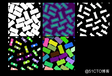
#%figonly=矩形区域分割算法各个步骤的输出图像
fig, axes = pl.subplots(2, 3, figsize=(7.5, 5.0), )
fig.delaxes(axes[1, 2])
axes[0, 0].imshow(squares, cmap="gray");
axes[0, 1].imshow(squares_dt)
axes[0, 2].imshow(squares_core, cmap="gray")
ax = axes[1, 0]
ax.imshow(cores)
center_y, center_x = centers.T
ax.plot(center_x, center_y, "o", color="white")
ax.set_xlim(0, w)
ax.set_ylim(h, 0)

axes[1, 1].imshow(separated)

for ax in axes.ravel():
ax.axis("off")

fig.subplots_adjust(wspace=0.01, hspace=0.01)

10.空间算法库-spatial

import numpy as np
import pylab as pl
from scipy import spatial

import matplotlib as mpl
mpl.rcParams['font.sans-serif'] = ['SimHei']

计算最近旁点

x = np.sort(np.random.rand(100))
idx = np.searchsorted(x, 0.5)
print (x[idx], x[idx - 1]) #距离0.5最近的数是这两个数中的一个

0.5244435681885733 0.4982156075770372

from scipy import spatial
np.random.seed(42)
N = 100
points = np.random.uniform(-1, 1, (N, 2))
kd = spatial.cKDTree(points)

targets = np.array([(0, 0), (0.5, 0.5), (-0.5, 0.5), (0.5, -0.5), (-0.5, -0.5)])
dist, idx = kd.query(targets, 3)

r = 0.2
idx2 = kd.query_ball_point(targets, r)
idx2

array([list([48]), list([37, 78]), list([22, 79, 92]), list([6, 35, 58]),
list([7, 42, 55, 83])], dtype=object)

idx3 = kd.query_pairs(0.1) - kd.query_pairs(0.08)
idx3

{(1, 46),
(3, 21),
(3, 82),
(3, 95),
(5, 16),
(9, 30),
(10, 87),
(11, 42),
(11, 97),
(18, 41),
(29, 74),
(32, 51),
(37, 78),
(39, 61),
(41, 61),
(50, 84),
(55, 83),
(73, 81)}

#%figonly=用cKDTree寻找近旁点
x, y = points.T
colors = "r", "b", "g", "y", "k"

fig, (ax1, ax2, ax3) = pl.subplots(1, 3, figsize=(12, 4))

for ax in ax1, ax2, ax3:
ax.set_aspect("equal")
ax.plot(x, y, "o", markersize=4)

for ax in ax1, ax2:
for i in range(len(targets)):
c = colors[i]
tx, ty = targets[i]
ax.plot([tx], [ty], "*", markersize=10, color=c)

for i in range(len(targets)):
nx, ny = points[idx[i]].T
ax1.plot(nx, ny, "o", markersize=10, markerfacecolor="None",
markeredgecolor=colors[i], markeredgewidth=1)

nx, ny = points[idx2[i]].T
ax2.plot(nx, ny, "o", markersize=10, markerfacecolor="None",
markeredgecolor=colors[i], markeredgewidth=1)

ax2.add_artist(pl.Circle(targets[i], r, fill=None, linestyle="dashed"))

for pidx1, pidx2 in idx3:
sx, sy = points[pidx1]
ex, ey = points[pidx2]
ax3.plot([sx, ex], [sy, ey], "r", linewidth=2, alpha=0.6)

ax1.set_xlabel(u"搜索最近的3个近旁点")
ax2.set_xlabel(u"搜索距离在0.2之内的所有近旁点")
ax3.set_xlabel(u"搜索所有距离在0.08到0.1之间的点对");

from scipy.spatial import distance
dist1 = distance.squareform(distance.pdist(points))
dist2 = distance.cdist(points, targets)
print(dist1.shape)
print(dist2.shape)

(100, 100)
(100, 5)

print (dist[:, 0]) # cKDTree.query()返回的与targets最近的距离
print (np.min(dist2, axis=0))

[0.15188266 0.09595807 0.05009422 0.11180181 0.19015485]
[0.15188266 0.09595807 0.05009422 0.11180181 0.19015485]

dist1[np.diag_indices(len(points))] = np.inf
nearest_pair = np.unravel_index(np.argmin(dist1), dist1.shape)
print (nearest_pair, dist1[nearest_pair])

(22, 92) 0.005346210248158245

dist, idx = kd.query(points, 2)
print (idx[np.argmin(dist[:, 1])], np.min(dist[:, 1]))

[22 92] 0.005346210248158245

N = 1000000
start = np.random.uniform(0, 100, N)
span = np.random.uniform(0.01, 1, N)
span = np.clip(span, 2, 100)
end = start + span

def naive_count_at(start, end, time):
mask = (start < time) & (end > time)
return np.sum(mask)

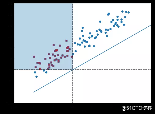
#%figonly=使用二维K-d树搜索指定区间的在线用户
def _():
N = 100
start = np.random.uniform(0, 100, N)
span = np.random.normal(40, 10, N)
span = np.clip(span, 2, 100)
end = start + span

time = 40

fig, ax = pl.subplots(figsize=(8, 6))
ax.scatter(start, end)
mask = (start < time) & (end > time)
start2, end2 = start[mask], end[mask]
ax.scatter(start2, end2, marker="x", color="red")
rect = pl.Rectangle((-20, 40), 60, 120, alpha=0.3)
ax.add_patch(rect)
ax.axhline(time, color="k", ls="--")
ax.axvline(time, color="k", ls="--")
ax.set_xlabel("Start")
ax.set_ylabel("End")
ax.set_xlim(-20, 120)
ax.set_ylim(-20, 160)
ax.plot([0, 120], [0, 120])

_()

class KdSearch(object):
def __init__(self, start, end, leafsize=10):
self.tree = spatial.cKDTree(np.c_[start, end], leafsize=leafsize)
self.max_time = np.max(end)

def count_at(self, time):
max_time = self.max_time
to_search = spatial.cKDTree([[time - max_time, time + max_time]])
return self.tree.count_neighbors(to_search, max_time, p=np.inf)

naive_count_at(start, end, 40) == KdSearch(start, end).count_at(40)

True

QUESTION

请读者研究点数N和leafsize参数与创建 K-d 树和搜索时间之间的关系。

凸包

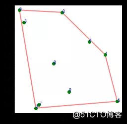
np.random.seed(42)
points2d = np.random.rand(10, 2)
ch2d = spatial.ConvexHull(points2d)
print(ch2d.simplices)
print(ch2d.vertices)

[[2 5]
[2 6]
[0 5]
[1 6]
[1 0]]
[5 2 6 1 0]

#%fig=二维平面上的凸包
poly = pl.Polygon(points2d[ch2d.vertices], fill=None, lw=2, color="r", alpha=0.5)
ax = pl.subplot(aspect="equal")
pl.plot(points2d[:, 0], points2d[:, 1], "go")
for i, pos in enumerate(points2d):
pl.text(pos[0], pos[1], str(i), color="blue")
ax.add_artist(poly);

np.random.seed(42)
points3d = np.random.rand(40, 3)
ch3d = spatial.ConvexHull(points3d)
ch3d.simplices.shape

(38, 3)

沃罗诺伊图

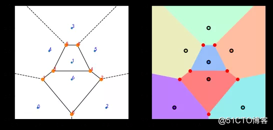
points2d = np.array([[0.2, 0.1], [0.5, 0.5], [0.8, 0.1],
[0.5, 0.8], [0.3, 0.6], [0.7, 0.6], [0.5, 0.35]])
vo = spatial.Voronoi(points2d)

print(vo.vertices); print(vo.regions); print(vo.ridge_vertices)

[[0.5 0.045 ]
[0.245 0.351 ]
[0.755 0.351 ]
[0.3375 0.425 ]
[0.6625 0.425 ]
[0.45 0.65 ]
[0.55 0.65 ]]
[[-1, 0, 1], [-1, 0, 2], [], [6, 4, 3, 5], [5, -1, 1, 3], [4, 2, 0, 1, 3], [6, -1, 2, 4], [6, -1, 5]]
[[-1, 0], [0, 1], [-1, 1], [0, 2], [-1, 2], [3, 5], [3, 4], [4, 6], [5, 6], [1, 3], [-1, 5], [2, 4], [-1, 6]]

bound = np.array([[-100, -100], [-100,  100],
[ 100,  100], [ 100, -100]])
vo2 = spatial.Voronoi(np.vstack((points2d, bound)))

#%figonly=沃罗诺伊图将空间分割为多个区域
fig, (ax1, ax2) = pl.subplots(1, 2, figsize=(9, 4.5))
ax1.set_aspect("equal")
ax2.set_aspect("equal")
spatial.voronoi_plot_2d(vo, ax=ax1)
for i, v in enumerate(vo.vertices):
ax1.text(v[0], v[1], str(i), color="red")

for i, p in enumerate(points2d):
ax1.text(p[0], p[1], str(i), color="blue")

n = len(points2d)
color = pl.cm.rainbow(np.linspace(0, 1, n))
for i in range(n):
idx = vo2.point_region[i]
region = vo2.regions[idx]
poly = pl.Polygon(vo2.vertices[region], facecolor=color[i], alpha=0.5, zorder=0)
ax2.add_artist(poly)
ax2.scatter(points2d[:, 0], points2d[:, 1], s=40, c=color, linewidths=2, edgecolors="k")
ax2.plot(vo2.vertices[:, 0], vo2.vertices[:, 1], "ro", ms=6)

for ax in ax1, ax2:
ax.set_xlim(0, 1)
ax.set_ylim(0, 1)

output_26_1

print (vo.point_region)
print (vo.regions[6])

[0 3 1 7 4 6 5]
[6, -1, 2, 4]

德劳内三角化

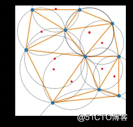
x = np.array([46.445, 263.251, 174.176, 280.899, 280.899,
189.358, 135.521, 29.638, 101.907, 226.665])
y = np.array([287.865, 250.891, 287.865, 160.975, 54.252,
160.975, 232.404, 179.187, 35.765, 71.361])
points2d = np.c_[x, y]
dy = spatial.Delaunay(points2d)
vo = spatial.Voronoi(points2d)
print(dy.simplices)
print(vo.vertices)

[[8 5 7]
[1 5 3]
[5 6 7]
[6 0 7]
[0 6 2]
[6 1 2]
[1 6 5]
[9 5 8]
[4 9 8]
[5 9 3]
[9 4 3]]
[[104.58977484 127.03566055]
[235.1285 198.68143374]
[107.83960707 155.53682482]
[ 71.22104881 228.39479887]
[110.3105 291.17642838]
[201.40695449 227.68436282]
[201.61895891 226.21958623]
[152.96231864 93.25060083]
[205.40381294 -90.5480267 ]
[235.1285 127.45701644]
[267.91709907 107.6135 ]]

#%fig=德劳内三角形的外接圆与圆心
cx, cy = vo.vertices.T

ax = pl.subplot(aspect="equal")
spatial.delaunay_plot_2d(dy, ax=ax)
ax.plot(cx, cy, "r.")
for i, (cx, cy) in enumerate(vo.vertices):
px, py = points2d[dy.simplices[i, 0]]
radius = np.hypot(cx - px, cy - py)
circle = pl.Circle((cx, cy), radius, fill=False, ls="dotted")
ax.add_artist(circle)
ax.set_xlim(0, 300)
ax.set_ylim(0, 300);