Paper:《Graph Neural Networks: A Review of Methods and Applications》翻译与解读
Paper:《Graph Neural Networks: A Review of Methods and Applications》翻译与解读
目录
《Graph Neural Networks: A Review of Methods and Applications》翻译与解读
2. Neural Networks as Relational Graphs
2.1. Message Exchange over Graphs
2.2. Fixed-width MLPs as Relational Graphs
2.3. General Neural Networks as Relational Graphs
3. Exploring Relational Graphs
3.1. Selection of Graph Measures
3.2. Design of Graph Generators
3.3. Controlling Computational Budget
4.2. Exploration with Relational Graphs
5.1. A Sweet Spot for Top Neural Networks
5.2. Neural Network Performance as a Smooth Function over Graph Measures
5.3. Consistency across Architectures
5.4. Quickly Identifying a Sweet Spot
5.5. Network Science and Neuroscience Connections
《Graph Neural Networks: A Review of Methods and Applications》翻译与解读
原论文地址:
https://arxiv.org/pdf/2007.06559.pdf
https://arxiv.org/abs/2007.06559
| Comments: |
ICML 2020 [Submitted on 13 Jul 2020] |
| Subjects: | Machine Learning (cs.LG); Computer Vision and Pattern Recognition (cs.CV); Social and Information Networks (cs.SI); Machine Learning (stat.ML) |
| Cite as: | arXiv:2007.06559 [cs.LG] (or arXiv:2007.06559v1 [cs.LG] for this version) |
Abstract
| Neural networks are often represented as graphs of connections between neurons. However, despite their wide use, there is currently little understanding of the relationship between the graph structure of the neural network and its predictive performance. Here we systematically investigate how does the graph structure of neural networks affect their predictive performance. To this end, we develop a novel graph-based representation of neural networks called relational graph, where layers of neural network computation correspond to rounds of message exchange along the graph structure. Using this representation we show that: (1) a "sweet spot" of relational graphs leads to neural networks with significantly improved predictive performance; (2) neural network's performance is approximately a smooth function of the clustering coefficient and average path length of its relational graph; (3) our findings are consistent across many different tasks and datasets; (4) the sweet spot can be identified efficiently; (5) top-performing neural networks have graph structure surprisingly similar to those of real biological neural networks. Our work opens new directions for the design of neural architectures and the understanding on neural networks in general. |
神经网络通常用神经元之间的连接图来表示。然而,尽管它们被广泛使用,目前人们对神经网络的图结构与其预测性能之间的关系知之甚少。在这里,我们系统地研究如何图结构的神经网络影响其预测性能。为此,我们开发了一种新的基于图的神经网络表示,称为关系图,其中神经网络计算的层对应于沿着图结构的消息交换轮数。利用这种表示法,我们证明:
|
1. Introduction
|
Deep neural networks consist of neurons organized into layers and connections between them. Architecture of a neural network can be captured by its “computational graph” where neurons are represented as nodes and directed edges link neurons in different layers. Such graphical representation demonstrates how the network passes and transforms the information from its input neurons, through hidden layers all the way to the output neurons (McClelland et al., 1986). While it has been widely observed that performance of neural networks depends on their architecture (LeCun et al., 1998; Krizhevsky et al., 2012; Simonyan & Zisserman, 2015; Szegedy et al., 2015; He et al., 2016), there is currently little systematic understanding on the relation between a neural network’s accuracy and its underlying graph structure. This is especially important for the neural architecture search, which today exhaustively searches over all possible connectivity patterns (Ying et al., 2019). From this perspective, several open questions arise:
Establishing such a relation is both scientifically and practically important because it would have direct consequences on designing more efficient and more accurate architectures. It would also inform the design of new hardware architectures that execute neural networks. Understanding the graph structures that underlie neural networks would also advance the science of deep learning. However, establishing the relation between network architecture and its accuracy is nontrivial, because it is unclear how to map a neural network to a graph (and vice versa). The natural choice would be to use computational graph representation but it has many limitations: (1) lack of generality: Computational graphs are constrained by the allowed graph properties, e.g., these graphs have to be directed and acyclic (DAGs), bipartite at the layer level, and single-in-single-out at the network level (Xie et al., 2019). This limits the use of the rich tools developed for general graphs. (2) Disconnection with biology/neuroscience: Biological neural networks have a much richer and less templatized structure (Fornito et al., 2013). There are information exchanges, rather than just single-directional flows, in the brain networks (Stringer et al., 2018). Such biological or neurological models cannot be simply represented by directed acyclic graphs. |
深层神经网络由神经元组成,这些神经元被组织成层,并在层与层之间建立联系。神经网络的结构可以通过它的“计算图”来捕获,其中神经元被表示为节点,有向边连接不同层次的神经元。这样的图形表示演示了网络如何传递和转换来自输入神经元的信息,通过隐藏层一直到输出神经元(McClelland et al., 1986)。虽然已广泛观察到神经网络的性能取决于其结构(LeCun et al., 1998;Krizhevsky等,2012;Simonyan & Zisserman, 2015;Szegedy等,2015;对于神经网络的精度与其底层图结构之间的关系,目前尚无系统的认识。这对于神经结构搜索来说尤为重要,如今,神经结构搜索遍寻所有可能的连通性模式(Ying等人,2019)。从这个角度来看,几个开放的问题出现了:
建立这样的关系在科学上和实践上都很重要,因为它将直接影响到设计更高效、更精确的架构。它还将指导执行神经网络的新硬件架构的设计。理解神经网络的图形结构也将推进深度学习科学。 然而,建立网络架构与其准确度之间的关系并非无关紧要,因为还不清楚如何将神经网络映射到图(反之亦然)。自然选择是使用计算图表示,但它有很多限制:(1)缺乏普遍性:计算图被限制允许图形属性,例如,这些图表必须指导和无环(无进取心的人),在层级别由两部分构成的,single-in-single-out在网络层(谢et al ., 2019)。这限制了为一般图形开发的丰富工具的使用。(2)与生物学/神经科学的分离:生物神经网络具有更丰富的、更少圣殿化的结构(Fornito et al., 2013)。大脑网络中存在着信息交换,而不仅仅是单向流动(Stringer et al., 2018)。这样的生物或神经模型不能简单地用有向无环图来表示。 |
|
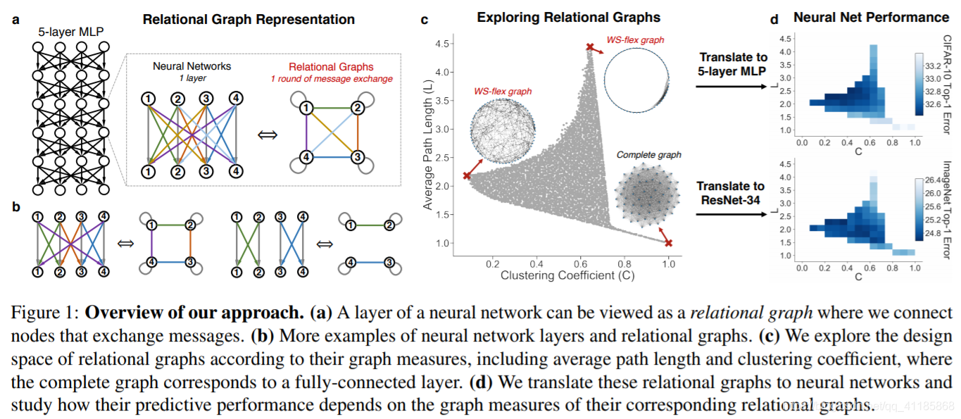
Here we systematically study the relationship between the graph structure of a neural network and its predictive performance. We develop a new way of representing a neural network as a graph, which we call relational graph. Our key insight is to focus on message exchange, rather than just on directed data flow. As a simple example, for a fixedwidth fully-connected layer, we can represent one input channel and one output channel together as a single node, and an edge in the relational graph represents the message exchange between the two nodes (Figure 1(a)). Under this formulation, using appropriate message exchange definition, we show that the relational graph can represent many types of neural network layers (a fully-connected layer, a convolutional layer, etc.), while getting rid of many constraints of computational graphs (such as directed, acyclic, bipartite, single-in-single-out). One neural network layer corresponds to one round of message exchange over a relational graph, and to obtain deep networks, we perform message exchange over the same graph for several rounds. Our new representation enables us to build neural networks that are richer and more diverse and analyze them using well-established tools of network science (Barabasi & Psfai ´ , 2016). We then design a graph generator named WS-flex that allows us to systematically explore the design space of neural networks (i.e., relation graphs). Based on the insights from neuroscience, we characterize neural networks by the clustering coefficient and average path length of their relational graphs (Figure 1(c)). Furthermore, our framework is flexible and general, as we can translate relational graphs into diverse neural architectures, including Multilayer Perceptrons (MLPs), Convolutional Neural Networks (CNNs), ResNets, etc. with controlled computational budgets (Figure 1(d)). |
本文系统地研究了神经网络的图结构与其预测性能之间的关系。我们提出了一种将神经网络表示为图的新方法,即关系图。我们的重点是关注消息交换,而不仅仅是定向数据流。作为一个简单的例子,对于固定宽度的全连接层,我们可以将一个输入通道和一个输出通道一起表示为单个节点,关系图中的一条边表示两个节点之间的消息交换(图1(a))。在此公式下,利用适当的消息交换定义,我们表明关系图可以表示多种类型的神经网络层(全连通层、卷积层等),同时摆脱了计算图的许多约束(如有向、无环、二部图、单入单出)。一个神经网络层对应于在关系图上进行一轮消息交换,为了获得深度网络,我们在同一图上进行几轮消息交换。我们的新表示使我们能够构建更加丰富和多样化的神经网络,并使用成熟的网络科学工具对其进行分析(Barabasi & Psfai, 2016)。 然后我们设计了一个名为WS-flex的图形生成器,它允许我们系统地探索神经网络的设计空间。关系图)。基于神经科学的见解,我们通过聚类系数和关系图的平均路径长度来描述神经网络(图1(c))。此外,我们的框架是灵活和通用的,因为我们可以将关系图转换为不同的神经结构,包括多层感知器(MLPs)、卷积神经网络(CNNs)、ResNets等,并控制计算预算(图1(d))。 |
|
Using standard image classification datasets CIFAR-10 and ImageNet, we conduct a systematic study on how the architecture of neural networks affects their predictive performance. We make several important empirical observations:
Our results have implications for designing neural network architectures, advancing the science of deep learning and improving our understanding of neural networks in general. |
使用标准图像分类数据集CIFAR-10和ImageNet,我们对神经网络的结构如何影响其预测性能进行了系统研究。我们做了几个重要的经验观察:
|
|
Figure 1: Overview of our approach. (a) A layer of a neural network can be viewed as a relational graph where we connect nodes that exchange messages. (b) More examples of neural network layers and relational graphs. (c) We explore the design space of relational graphs according to their graph measures, including average path length and clustering coefficient, where the complete graph corresponds to a fully-connected layer. (d) We translate these relational graphs to neural networks and study how their predictive performance depends on the graph measures of their corresponding relational graphs. 图1:我们方法的概述。(a)神经网络的一层可以看作是一个关系图,在这里我们连接交换消息的节点。(b)神经网络层和关系图的更多例子。(c)我们根据关系图的图度量来探索关系图的设计空间,包括平均路径长度和聚类系数,其中完全图对应一个全连通层。我们将这些关系图转换为神经网络,并研究它们的预测性能如何取决于对应关系图的图度量。 |
2. Neural Networks as Relational Graphs
| To explore the graph structure of neural networks, we first introduce the concept of our relational graph representation and its instantiations. We demonstrate how our representation can capture diverse neural network architectures under a unified framework. Using the language of graph in the context of deep learning helps bring the two worlds together and establish a foundation for our study. |
为了探讨神经网络的图结构,我们首先介绍关系图表示的概念及其实例。我们将演示如何在统一框架下捕获不同的神经网络架构。在深度学习的背景下使用graph语言有助于将这两个世界结合起来,为我们的研究奠定基础。 |
2.1. Message Exchange over Graphs
|
We start by revisiting the definition of a neural network from the graph perspective. We define a graph G = (V, E) by its node set V = {v1, ..., vn} and edge set E ⊆ {(vi , vj )|vi , vj ∈ V}. We assume each node v has a node feature scalar/vector xv.
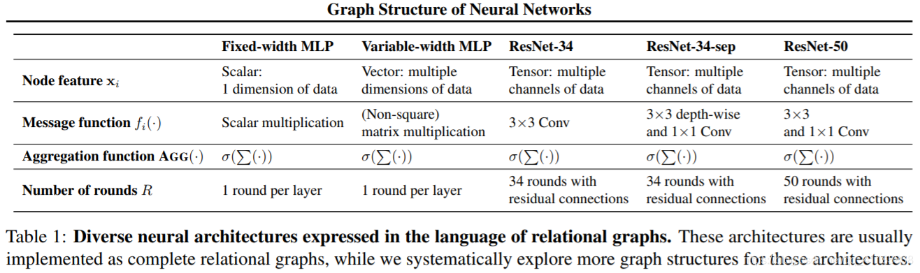
Table 1: Diverse neural architectures expressed in the language of relational graphs. These architectures are usually implemented as complete relational graphs, while we systematically explore more graph structures for these architectures. 表1:用关系图语言表示的各种神经结构。这些架构通常被实现为完整的关系图,而我们系统地为这些架构探索更多的图结构。
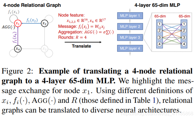
Figure 2: Example of translating a 4-node relational graph to a 4-layer 65-dim MLP. We highlight the message exchange for node x1. Using different definitions of xi , fi(·), AGG(·) and R (those defined in Table 1), relational graphs can be translated to diverse neural architectures. 图2:将4节点关系图转换为4层65-dim MLP的示例。我们将重点介绍节点x1的消息交换。使用xi、fi(·)、AGG(·)和R(表1中定义的)的不同定义,关系图可以转换为不同的神经结构。 |
|
|
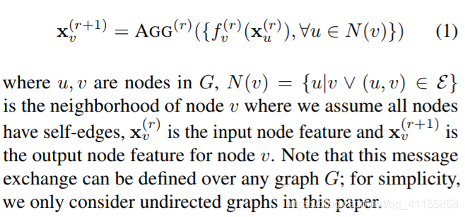
We call graph G a relational graph, when it is associated with message exchanges between neurons. Specifically, a message exchange is defined by a message function, whose input is a node’s feature and output is a message, and an aggregation function, whose input is a set of messages and output is the updated node feature. At each round of message exchange, each node sends messages to its neighbors, and aggregates incoming messages from its neighbors. Each message is transformed at each edge through a message function f(·), then they are aggregated at each node via an aggregation function AGG(·). Suppose we conduct R rounds of message exchange, then the r-th round of message exchange for a node v can be described as
Equation 1 provides a general definition for message exchange. In the remainder of this section, we discuss how this general message exchange definition can be instantiated as different neural architectures. We summarize the different instantiations in Table 1, and provide a concrete example of instantiating a 4-layer 65-dim MLP in Figure 2. |
我们称图G为关系图,当它与神经元之间的信息交换有关时。具体来说,消息交换由消息函数和聚合函数定义,前者的输入是节点的特性,输出是消息,后者的输入是一组消息,输出是更新后的节点特性。在每一轮消息交换中,每个节点向它的邻居发送消息,并聚合从它的邻居传入的消息。每个消息通过消息函数f(·)在每个边进行转换,然后通过聚合函数AGG(·)在每个节点进行聚合。假设我们进行了R轮的消息交换,那么节点v的第R轮消息交换可以描述为 公式1提供了消息交换的一般定义。在本节的其余部分中,我们将讨论如何将这个通用消息交换定义实例化为不同的神经结构。我们在表1中总结了不同的实例,并在图2中提供了实例化4层65-dim MLP的具体示例。 |
2.2. Fixed-width MLPs as Relational Graphs
|
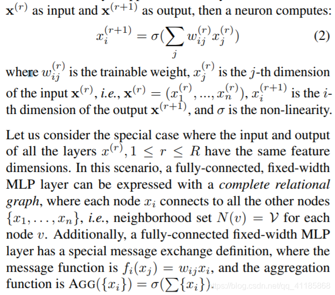
A Multilayer Perceptron (MLP) consists of layers of computation units (neurons), where each neuron performs a weighted sum over scalar inputs and outputs, followed by some non-linearity. Suppose the r-th layer of an MLP takes x (r) as input and x (r+1) as output, then a neuron computes:
|
一个多层感知器(MLP)由多层计算单元(神经元)组成,其中每个神经元执行标量输入和输出的加权和,然后是一些非线性。假设MLP的第r层以x (r)为输入,x (r+1)为输出,则有一个神经元计算: |
|
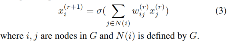
The above discussion reveals that a fixed-width MLP can be viewed as a complete relational graph with a special message exchange function. Therefore, a fixed-width MLP is a special case under a much more general model family, where the message function, aggregation function, and most importantly, the relation graph structure can vary. This insight allows us to generalize fixed-width MLPs from using complete relational graph to any general relational graph G. Based on the general definition of message exchange in Equation 1, we have:
|
上面的讨论表明,可以将固定宽度的MLP视为具有特殊消息交换功能的完整关系图。因此,固定宽度的MLP是更为通用的模型系列中的一种特殊情况,其中消息函数、聚合函数以及最重要的关系图结构可能会发生变化。 这使得我们可以将固定宽度MLPs从使用完全关系图推广到任何一般关系图g。根据公式1中消息交换的一般定义,我们有: |
2.3. General Neural Networks as Relational Graphs
|
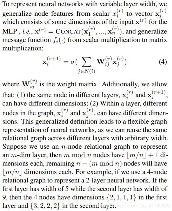
The graph viewpoint in Equation 3 lays the foundation of representing fixed-width MLPs as relational graphs. In this section, we discuss how we can further generalize relational graphs to general neural networks. Variable-width MLPs as relational graphs. An important design consideration for general neural networks is that layer width often varies through out the network. For example, in CNNs, a common practice is to double the layer width (number of feature channels) after spatial down-sampling.
|
式3中的图点为将定宽MLPs表示为关系图奠定了基础。在这一节中,我们将讨论如何进一步将关系图推广到一般的神经网络。 可变宽度MLPs作为关系图。对于一般的神经网络,一个重要的设计考虑是网络的层宽经常是不同的。例如,在CNNs中,常用的做法是在空间下采样后将层宽(特征通道数)增加一倍。 |
|
Note that under this definition, the maximum number of nodes of a relational graph is bounded by the width of the narrowest layer in the corresponding neural network (since the feature dimension for each node must be at least 1).
|
注意,在这个定义下,关系图的最大节点数以对应神经网络中最窄层的宽度为界(因为每个节点的特征维数必须至少为1)。 |
|
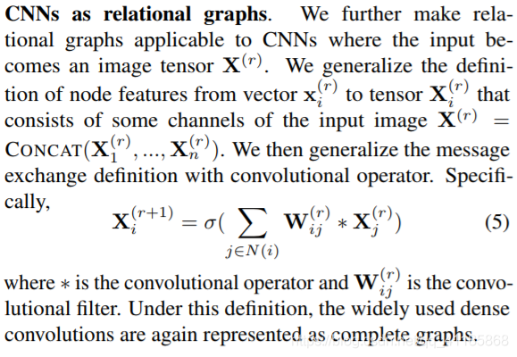
Modern neural architectures as relational graphs. Finally, we generalize relational graphs to represent modern neural architectures with more sophisticated designs. For example, to represent a ResNet (He et al., 2016), we keep the residual connections between layers unchanged. To represent neural networks with bottleneck transform (He et al., 2016), a relational graph alternatively applies message exchange with 3×3 and 1×1 convolution; similarly, in the efficient computing setup, the widely used separable convolution (Howard et al., 2017; Chollet, 2017) can be viewed as alternatively applying message exchange with 3×3 depth-wise convolution and 1×1 convolution. Overall, relational graphs provide a general representation for neural networks. With proper definitions of node features and message exchange, relational graphs can represent diverse neural architectures, as is summarized in Table 1. |
作为关系图的现代神经结构。最后,我们推广了关系图,用更复杂的设计来表示现代神经结构。例如,为了表示ResNet (He et al., 2016),我们保持层之间的剩余连接不变。为了用瓶颈变换表示神经网络(He et al., 2016),关系图交替应用3×3和1×1卷积的消息交换;同样,在高效的计算设置中,广泛使用的可分离卷积(Howard et al., 2017;Chollet, 2017)可以看作是3×3深度卷积和1×1卷积交替应用消息交换。 总的来说,关系图提供了神经网络的一般表示。通过正确定义节点特性和消息交换,关系图可以表示不同的神经结构,如表1所示。 |
3. Exploring Relational Graphs
| In this section, we describe in detail how we design and explore the space of relational graphs defined in Section 2, in order to study the relationship between the graph structure of neural networks and their predictive performance. Three main components are needed to make progress: (1) graph measures that characterize graph structural properties, (2) graph generators that can generate diverse graphs, and (3) a way to control the computational budget, so that the differences in performance of different neural networks are due to their diverse relational graph structures. |
在本节中,我们将详细描述如何设计和探索第二节中定义的关系图空间,以研究神经网络的图结构与其预测性能之间的关系。三个主要组件是需要取得进展:(1)图的措施描述图的结构性质,(2)图形发生器,可以产生不同的图表,和(3)一种方法来控制计算预算,以便不同神经网络的性能的差异是由于各自不同的关系图结构。 |
3.1. Selection of Graph Measures
| Given the complex nature of graph structure, graph measures are often used to characterize graphs. In this paper, we focus on one global graph measure, average path length, and one local graph measure, clustering coefficient. Notably, these two measures are widely used in network science (Watts & Strogatz, 1998) and neuroscience (Sporns, 2003; Bassett & Bullmore, 2006). Specifically, average path length measures the average shortest path distance between any pair of nodes; clustering coefficient measures the proportion of edges between the nodes within a given node’s neighborhood, divided by the number of edges that could possibly exist between them, averaged over all the nodes. There are other graph measures that can be used for analysis, which are included in the Appendix. |
由于图结构的复杂性,图测度通常被用来刻画图的特征。本文主要研究了一个全局图测度,即平均路径长度,和一个局部图测度,即聚类系数。值得注意的是,这两种方法在网络科学(Watts & Strogatz, 1998)和神经科学(Sporns, 2003;巴西特和布尔莫尔,2006年)。具体来说,平均路径长度度量任意对节点之间的平均最短路径距离;聚类系数度量给定节点邻域内节点之间的边的比例,除以它们之间可能存在的边的数量,平均到所有节点上。还有其他可以用于分析的图表度量,包括在附录中。 |
3.2. Design of Graph Generators
|
Given selected graph measures, we aim to generate diverse graphs that can cover a large span of graph measures, using a graph generator. However, such a goal requires careful generator designs: classic graph generators can only generate a limited class of graphs, while recent learning-based graph generators are designed to imitate given exemplar graphs (Kipf & Welling, 2017; Li et al., 2018b; You et al., 2018a;b; 2019a). Limitations of existing graph generators. To illustrate the limitation of existing graph generators, we investigate the following classic graph generators: (1) Erdos-R ˝ enyi ´ (ER) model that can sample graphs with given node and edge number uniformly at random (Erdos & R ˝ enyi ´ , 1960); (2) Watts-Strogatz (WS) model that can generate graphs with small-world properties (Watts & Strogatz, 1998); (3) Barabasi-Albert (BA) model that can generate scale-free ´ graphs (Albert & Barabasi ´ , 2002); (4) Harary model that can generate graphs with maximum connectivity (Harary, 1962); (5) regular ring lattice graphs (ring graphs); (6) complete graphs. For all types of graph generators, we control the number of nodes to be 64, enumerate all possible discrete parameters and grid search over all continuous parameters of the graph generator. We generate 30 random graphs with different random seeds under each parameter setting. In total, we generate 486,000 WS graphs, 53,000 ER graphs, 8,000 BA graphs, 1,800 Harary graphs, 54 ring graphs and 1 complete graph (more details provided in the Appendix). In Figure 3, we can observe that graphs generated by those classic graph generators have a limited span in the space of average path length and clustering coefficient. |
给定选定的图度量,我们的目标是使用图生成器生成能够覆盖大范围图度量的不同图。然而,这样的目标需要仔细的生成器设计:经典的图形生成器只能生成有限的图形类,而最近的基于学习的图形生成器被设计用来模仿给定的范例图形(Kipf & Welling, 2017;李等,2018b;You等,2018a;b;2019年)。 现有图形生成器的局限性。为了说明现有图生成器的限制,我们调查以下经典图生成器:(1)可以随机统一地用给定节点和边数采样图的厄多斯-R图表生成器(厄多斯& R他们是在1960年);(2)能够生成具有小世界特性图的Watts-Strogatz (WS)模型(Watts & Strogatz, 1998);(3) barabsi -Albert (BA)模型,可以生成无尺度的’图(Albert & Barabasi, 2002);(4)可生成最大连通性图的Harary模型(Harary, 1962);(5)正则环格图(环图);(6)完成图表。对于所有类型的图生成器,我们控制节点数为64,枚举所有可能的离散参数,并对图生成器的所有连续参数进行网格搜索。我们在每个参数设置下生成30个带有不同随机种子的随机图。总共生成486,000个WS图、53,000个ER图、8,000个BA图、1,800个Harary图、54个环图和1个完整图(详情见附录)。在图3中,我们可以看到经典的图生成器生成的图在平均路径长度和聚类系数的空间中具有有限的跨度。
|
| WS-flex graph generator. Here we propose the WS-flex graph generator that can generate graphs with a wide coverage of graph measures; notably, WS-flex graphs almost encompass all the graphs generated by classic random generators mentioned above, as is shown in Figure 3. WSflex generator generalizes WS model by relaxing the constraint that all the nodes have the same degree before random rewiring. Specifically, WS-flex generator is parametrized by node n, average degree k and rewiring probability p. The number of edges is determined as e = bn ∗ k/2c. Specifically, WS-flex generator first creates a ring graph where each node connects to be/nc neighboring nodes; then the generator randomly picks e mod n nodes and connects each node to one closest neighboring node; finally, all the edges are randomly rewired with probability p. We use WS-flex generator to smoothly sample within the space of clustering coefficient and average path length, then sub-sample 3942 graphs for our experiments, as is shown in Figure 1(c). | WS-flex图生成器。在这里,我们提出了WS-flex图形生成器,它可以生成覆盖范围广泛的图形度量;值得注意的是,WS-flex图几乎包含了上面提到的经典随机生成器生成的所有图,如图3所示。WSflex生成器是对WS模型的一般化,它放宽了随机重新布线前所有节点具有相同程度的约束。具体来说,WS-flex生成器由节点n、平均度k和重新布线概率p参数化。边的数量确定为e = bn∗k/2c。具体来说,WS-flex生成器首先创建一个环图,其中每个节点连接到be/nc相邻节点;然后随机选取e mod n个节点,将每个节点连接到一个最近的相邻节点;最后,以概率p随机重新连接所有的边。我们使用WS-flex生成器在聚类系数和平均路径长度的空间内平滑采样,然后进行我们实验的子样本3942张图,如图1(c)所示。 |
3.3. Controlling Computational Budget
|
To compare the neural networks translated by these diverse graphs, it is important to ensure that all networks have approximately the same complexity, so that the differences in performance are due to their relational graph structures. We use FLOPS (# of multiply-adds) as the metric. We first compute the FLOPS of our baseline network instantiations (i.e. complete relational graph), and use them as the reference complexity in each experiment. As described in Section 2.3, a relational graph structure can be instantiated as a neural network with variable width, by partitioning dimensions or channels into disjoint set of node features. Therefore, we can conveniently adjust the width of a neural network to match the reference complexity (within 0.5% of baseline FLOPS) without changing the relational graph structures. We provide more details in the Appendix.
|
为了比较由这些不同图转换的神经网络,确保所有网络具有近似相同的复杂性是很重要的,这样性能上的差异是由于它们的关系图结构造成的。我们使用FLOPS (number of multiply- added)作为度量标准。我们首先计算我们的基线网络实例化的失败(即完全关系图),并使用它们作为每个实验的参考复杂度。如2.3节所述,通过将维度或通道划分为节点特征的不相交集,可以将关系图结构实例化为宽度可变的神经网络。因此,我们可以方便地调整神经网络的宽度,以匹配参考复杂度(在基线失败的0.5%以内),而不改变关系图结构。我们在附录中提供了更多细节。 |

4. Experimental Setup
| Considering the large number of candidate graphs (3942 in total) that we want to explore, we first investigate graph structure of MLPs on the CIFAR-10 dataset (Krizhevsky, 2009) which has 50K training images and 10K validation images. We then further study the larger and more complex task of ImageNet classification (Russakovsky et al., 2015), which consists of 1K image classes, 1.28M training images and 50K validation images. |
考虑到我们想要探索的候选图数量很大(总共3942个),我们首先在CIFAR-10数据集(Krizhevsky, 2009)上研究MLPs的图结构,该数据集有50K训练图像和10K验证图像。然后,我们进一步研究了更大、更复杂的ImageNet分类任务(Russakovsky et al., 2015),包括1K图像类、1.28M训练图像和50K验证图像。 |
4.1. Base Architectures
| For CIFAR-10 experiments, We use a 5-layer MLP with 512 hidden units as the baseline architecture. The input of the MLP is a 3072-d flattened vector of the (32×32×3) image, the output is a 10-d prediction. Each MLP layer has a ReLU non-linearity and a BatchNorm layer (Ioffe & Szegedy, 2015). We train the model for 200 epochs with batch size 128, using cosine learning rate schedule (Loshchilov & Hutter, 2016) with an initial learning rate of 0.1 (annealed to 0, no restarting). We train all MLP models with 5 different random seeds and report the averaged results. | 在CIFAR-10实验中,我们使用一个5层的MLP和512个隐藏单元作为基线架构 20a29 。MLP的输入是(32×32×3)图像的3072 d平坦向量,输出是10 d预测。每个MLP层具有ReLU非线性和BatchNorm层(Ioffe & Szegedy, 2015)。我们使用余弦学习率计划(Loshchilov & Hutter, 2016)训练批量大小为128的200个epoch的模型,初始学习率为0.1(退火到0,不重新启动)。我们用5种不同的随机种子训练所有的MLP模型,并报告平均结果。 |
| For ImageNet experiments, we use three ResNet-family architectures, including (1) ResNet-34, which only consists of basic blocks of 3×3 convolutions (He et al., 2016); (2) ResNet-34-sep, a variant where we replace all 3×3 dense convolutions in ResNet-34 with 3×3 separable convolutions (Chollet, 2017); (3) ResNet-50, which consists of bottleneck blocks (He et al., 2016) of 1×1, 3×3, 1×1 convolutions. Additionally, we use EfficientNet-B0 architecture (Tan & Le, 2019) that achieves good performance in the small computation regime. Finally, we use a simple 8- layer CNN with 3×3 convolutions. The model has 3 stages with [64, 128, 256] hidden units. Stride-2 convolutions are used for down-sampling. The stem and head layers are the same as a ResNet. We train all the ImageNet models for 100 epochs using cosine learning rate schedule with initial learning rate of 0.1. Batch size is 256 for ResNetfamily models and 512 for EfficientNet-B0. We train all ImageNet models with 3 random seeds and report the averaged performance. All the baseline architectures have a complete relational graph structure. The reference computational complexity is 2.89e6 FLOPS for MLP, 3.66e9 FLOPS for ResNet-34, 0.55e9 FLOPS for ResNet-34-sep, 4.09e9 FLOPS for ResNet-50, 0.39e9 FLOPS for EffcientNet-B0, and 0.17e9 FLOPS for 8-layer CNN. Training an MLP model roughly takes 5 minutes on a NVIDIA Tesla V100 GPU, and training a ResNet model on ImageNet roughly takes a day on 8 Tesla V100 GPUs with data parallelism. We provide more details in Appendix. | 在ImageNet实验中,我们使用了三种resnet系列架构,包括(1)ResNet-34,它只包含3×3卷积的基本块(He et al., 2016);(2) ResNet-34-sep,将ResNet-34中的所有3×3稠密卷积替换为3×3可分离卷积(Chollet, 2017);(3) ResNet-50,由1×1,3×3,1×1卷积的瓶颈块(He et al., 2016)组成。此外,我们使用了efficiency - net - b0架构(Tan & Le, 2019),在小计算环境下取得了良好的性能。最后,我们使用一个简单的8层CNN, 3×3卷积。模型有3个阶段,隐含单元为[64,128,256]。Stride-2卷积用于下采样。茎和头层与ResNet相同。我们使用初始学习率为0.1的余弦学习率计划对所有ImageNet模型进行100个epoch的训练。批大小是256的ResNetfamily模型和512的效率网- b0。我们用3个随机种子训练所有的ImageNet模型,并报告平均性能。所有的基线架构都有一个完整的关系图结构。MLP的参考计算复杂度是2.89e6失败,ResNet-34的3.66e9失败,ResNet-34-sep的0.55e9失败,ResNet-50的4.09e9失败,EffcientNet-B0的0.39e9失败,8层CNN的0.17e9失败。在NVIDIA Tesla V100 GPU上训练一个MLP模型大约需要5分钟,而在ImageNet上训练一个ResNet模型大约需要一天,在8个Tesla V100 GPU上使用数据并行。我们在附录中提供更多细节。 |
|
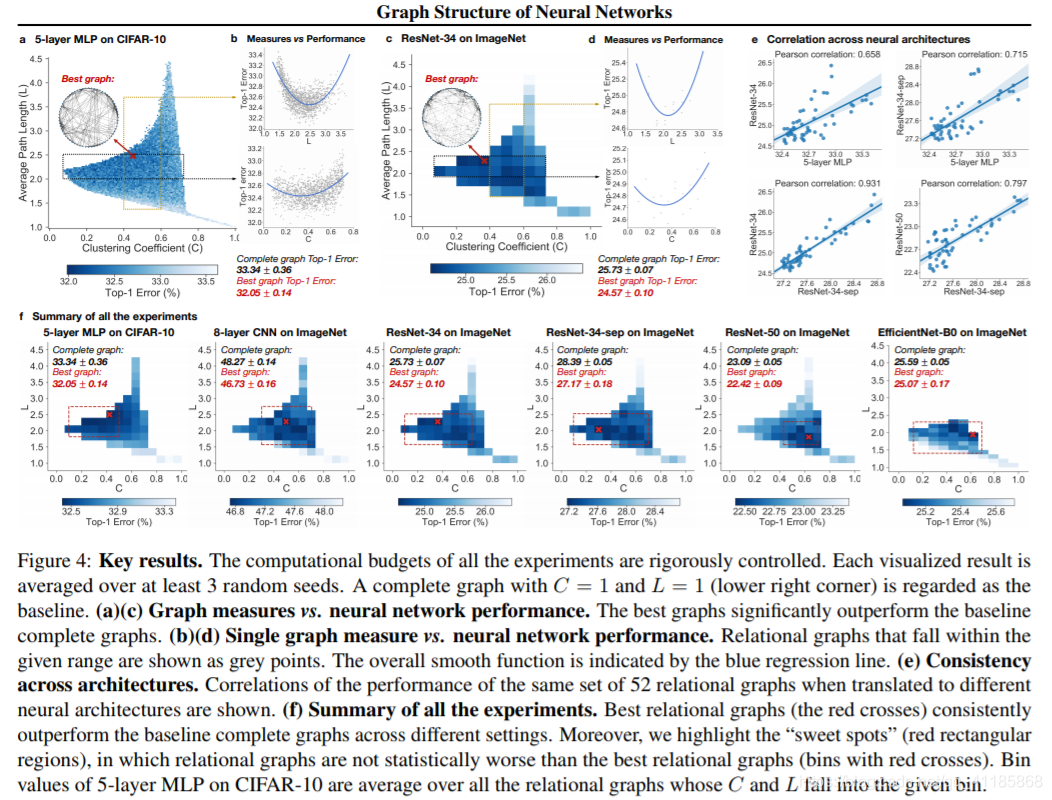
Figure 4: Key results. The computational budgets of all the experiments are rigorously controlled. Each visualized result is averaged over at least 3 random seeds. A complete graph with C = 1 and L = 1 (lower right corner) is regarded as the baseline. (a)(c) Graph measures vs. neural network performance. The best graphs significantly outperform the baseline complete graphs. (b)(d) Single graph measure vs. neural network performance. Relational graphs that fall within the given range are shown as grey points. The overall smooth function is indicated by the blue regression line. (e) Consistency across architectures. Correlations of the performance of the same set of 52 relational graphs when translated to different neural architectures are shown. (f) Summary of all the experiments. Best relational graphs (the red crosses) consistently outperform the baseline complete graphs across different settings. Moreover, we highlight the “sweet spots” (red rectangular regions), in which relational graphs are not statistically worse than the best relational graphs (bins with red crosses). Bin values of 5-layer MLP on CIFAR-10 are average over all the relational graphs whose C and L fall into the given bin 图4:关键结果。所有实验的计算预算都是严格控制的。每个可视化结果至少在3个随机种子上取平均值。以C = 1, L = 1(右下角)的完整图作为基线。(a)(c)图形测量与神经网络性能。最好的图表明显优于基线完整的图表。(b)(d)单图测量与神经网络性能。在给定范围内的关系图显示为灰色点。整体平滑函数用蓝色回归线表示。(e)架构之间的一致性。当转换到不同的神经结构时,同一组52个关系图的性能的相关性被显示出来。(f)总结所有实验。在不同的设置中,最佳关系图(红色叉)的表现始终优于基线完整图。此外,我们强调了“甜蜜点”(红色矩形区域),其中关系图在统计上并不比最佳关系图(红色叉的箱子)差。CIFAR-10上5层MLP的Bin值是C和L属于给定Bin的所有关系图的平均值 |
4.2. Exploration with Relational Graphs
|
For all the architectures, we instantiate each sampled relational graph as a neural network, using the corresponding definitions outlined in Table 1. Specifically, we replace all the dense layers (linear layers, 3×3 and 1×1 convolution layers) with their relational graph counterparts. We leave the input and output layer unchanged and keep all the other designs (such as down-sampling, skip-connections, etc.) intact. We then match the reference computational complexity for all the models, as discussed in Section 3.3. |
对于所有的架构,我们使用表1中列出的相应定义将每个抽样的关系图实例化为一个神经网络。具体来说,我们将所有的稠密层(线性层、3×3和1×1卷积层)替换为对应的关系图。我们保持输入和输出层不变,并保持所有其他设计(如下采样、跳接等)不变。然后我们匹配所有模型的参考计算复杂度,如3.3节所讨论的。 |
| For CIFAR-10 MLP experiments, we study 3942 sampled relational graphs of 64 nodes as described in Section 3.2. For ImageNet experiments, due to high computational cost, we sub-sample 52 graphs uniformly from the 3942 graphs. Since EfficientNet-B0 is a small model with a layer that has only 16 channels, we can not reuse the 64-node graphs sampled for other setups. We re-sample 48 relational graphs with 16 nodes following the same procedure in Section 3. |
对于CIFAR-10 MLP实验,我们研究了包含64个节点的3942个抽样关系图,如3.2节所述。在ImageNet实验中,由于计算量大,我们从3942个图中均匀地抽取52个图。因为efficient - b0是一个只有16个通道的层的小模型,我们不能在其他设置中重用64节点图。我们按照第3节中相同的步骤,对48个有16个节点的关系图重新采样。 |
5. Results
| In this section, we summarize the results of our experiments and discuss our key findings. We collect top-1 errors for all the sampled relational graphs on different tasks and architectures, and also record the graph measures (average path length L and clustering coefficient C) for each sampled graph. We present these results as heat maps of graph measures vs. predictive performance (Figure 4(a)(c)(f)). |
在本节中,我们将总结我们的实验结果并讨论我们的主要发现。我们收集了不同任务和架构上的所有抽样关系图的top-1错误,并记录了每个抽样图的图度量(平均路径长度L和聚类系数C)。我们将这些结果作为图表测量与预测性能的热图(图4(a)(c)(f))。 |
5.1. A Sweet Spot for Top Neural Networks
| Overall, the heat maps of graph measures vs. predictive performance (Figure 4(f)) show that there exist graph structures that can outperform the complete graph (the pixel on bottom right) baselines. The best performing relational graph can outperform the complete graph baseline by 1.4% top-1 error on CIFAR-10, and 0.5% to 1.2% for models on ImageNet. Notably, we discover that top-performing graphs tend to cluster into a sweet spot in the space defined by C and L (red rectangles in Figure 4(f)). We follow these steps to identify a sweet spot: (1) we downsample and aggregate the 3942 graphs in Figure 4(a) into a coarse resolution of 52 bins, where each bin records the performance of graphs that fall into the bin; (2) we identify the bin with best average performance (red cross in Figure 4(f)); (3) we conduct onetailed t-test over each bin against the best-performing bin, and record the bins that are not significantly worse than the best-performing bin (p-value 0.05 as threshold). The minimum area rectangle that covers these bins is visualized as a sweet spot. For 5-layer MLP on CIFAR-10, the sweet spot is C ∈ [0.10, 0.50], L ∈ [1.82, 2.75]. | 总的来说,图度量与预测性能的热图(图4(f))表明,存在的图结构可以超过整个图(右下角的像素)基线。在CIFAR-10中,表现最好的关系图的top-1误差比整个图基线高出1.4%,而在ImageNet中,模型的top-1误差为0.5%到1.2%。值得注意的是,我们发现性能最好的图往往聚集在C和L定义的空间中的一个最佳点(图4(f)中的红色矩形)。我们按照以下步骤来确定最佳点:(1)我们向下采样并将图4(a)中的3942个图汇总为52个大致分辨率的bin,每个bin记录落入bin的图的性能;(2)我们确定平均性能最佳的bin(图4(f)中的红十字会);(3)对每个箱子与性能最好的箱子进行最小t检验,记录性能不明显差的箱子(p-value 0.05为阈值)。覆盖这些箱子的最小面积矩形被可视化为一个甜点点。对于CIFAR-10上的5层MLP,最优点C∈[0.10,0.50],L∈[1.82,2.75]。 |
5.2. Neural Network Performance as a Smooth Function over Graph Measures
| In Figure 4(f), we observe that neural network’s predictive performance is approximately a smooth function of the clustering coefficient and average path length of its relational graph. Keeping one graph measure fixed in a small range (C ∈ [0.4, 0.6], L ∈ [2, 2.5]), we visualize network performances against the other measure (shown in Figure 4(b)(d)). We use second degree polynomial regression to visualize the overall trend. We observe that both clustering coefficient and average path length are indicative of neural network performance, demonstrating a smooth U-shape correlation |
在图4(f)中,我们观察到神经网络的预测性能近似是其聚类系数和关系图平均路径长度的平滑函数。将一个图度量固定在一个小范围内(C∈[0.4,0.6],L∈[2,2.5]),我们将网络性能与另一个度量进行可视化(如图4(b)(d)所示)。我们使用二次多项式回归来可视化总体趋势。我们观察到,聚类系数和平均路径长度都是神经网络性能的指标,呈平滑的u形相关 |
5.3. Consistency across Architectures
|
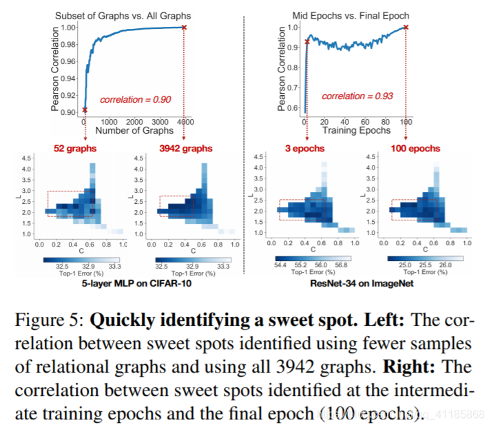
Figure 5: Quickly identifying a sweet spot. Left: The correlation between sweet spots identified using fewer samples of relational graphs and using all 3942 graphs. Right: The correlation between sweet spots identified at the intermediate training epochs and the final epoch (100 epochs). |
图5:快速确定最佳点。左图:使用较少的关系图样本和使用全部3942幅图识别出的甜点之间的相关性。右图:中间训练时期和最后训练时期(100个时期)确定的甜蜜点之间的相关性。 |
|
Given that relational graph defines a shared design space across various neural architectures, we observe that relational graphs with certain graph measures may consistently perform well regardless of how they are instantiated. Qualitative consistency. We visually observe in Figure 4(f) that the sweet spots are roughly consistent across different architectures. Specifically, if we take the union of the sweet spots across architectures, we have C ∈ [0.43, 0.50], L ∈ [1.82, 2.28] which is the consistent sweet spot across architectures. Moreover, the U-shape trends between graph measures and corresponding neural network performance, shown in Figure 4(b)(d), are also visually consistent. Quantitative consistency. To further quantify this consistency across tasks and architectures, we select the 52 bins in the heat map in Figure 4(f), where the bin value indicates the average performance of relational graphs whose graph measures fall into the bin range. We plot the correlation of the 52 bin values across different pairs of tasks, shown in Figure 4(e). We observe that the performance of relational graphs with certain graph measures correlates across different tasks and architectures. For example, even though a ResNet-34 has much higher complexity than a 5-layer MLP, and ImageNet is a much more challenging dataset than CIFAR-10, a fixed set relational graphs would perform similarly in both settings, indicated by a Pearson correlation of 0.658 (p-value < 10−8 ). |
假设关系图定义了跨各种神经结构的共享设计空间,我们观察到,无论如何实例化,具有特定图度量的关系图都可以始终执行得很好。 定性的一致性。在图4(f)中,我们可以直观地看到,不同架构之间的甜点点基本上是一致的。具体来说,如果我们取跨架构的甜蜜点的并集,我们有C∈[0.43,0.50],L∈[1.82,2.28],这是跨架构的一致的甜蜜点。此外,图4(b)(d)所示的图测度与对应的神经网络性能之间的u形趋势在视觉上也是一致的。 量化一致性。为了进一步量化跨任务和架构的一致性,我们在图4(f)的热图中选择了52个bin,其中bin值表示图度量在bin范围内的关系图的平均性能。我们绘制52个bin值在不同任务对之间的相关性,如图4(e)所示。我们观察到,具有特定图形的关系图的性能度量了不同任务和架构之间的关联。例如,尽管ResNet-34比5层MLP复杂得多,ImageNet是一个比ciremote -10更具挑战性的数据集,一个固定的集合关系图在两种设置中表现相似,通过0.658的Pearson相关性表示(p值< 10−8)。 |
5.4. Quickly Identifying a Sweet Spot
|
Training thousands of relational graphs until convergence might be computationally prohibitive. Therefore, we quantitatively show that a sweet spot can be identified with much less computational cost, e.g., by sampling fewer graphs and training for fewer epochs. How many graphs are needed? Using the 5-layer MLP on CIFAR-10 as an example, we consider the heat map over 52 bins in Figure 4(f) which is computed using 3942 graph samples. We investigate if a similar heat map can be produced with much fewer graph samples. Specifically, we sub-sample the graphs in each bin while making sure each bin has at least one graph. We then compute the correlation between the 52 bin values computed using all 3942 graphs and using sub-sampled fewer graphs, as is shown in Figure 5 (left). We can see that bin values computed using only 52 samples have a high 0.90 Pearson correlation with the bin values computed using full 3942 graph samples. This finding suggests that, in practice, much fewer graphs are needed to conduct a similar analysis. |
训练成千上万的关系图,直到运算上无法收敛为止。因此,我们定量地表明,可以用更少的计算成本来确定一个最佳点,例如,通过采样更少的图和训练更少的epoch。 需要多少个图?以CIFAR-10上的5层MLP为例,我们考虑图4(f)中52个箱子上的热图,该热图使用3942个图样本计算。我们研究了是否可以用更少的图表样本制作类似的热图。具体来说,我们对每个容器中的图进行子采样,同时确保每个容器至少有一个图。然后,我们计算使用所有3942图和使用更少的次采样图计算的52个bin值之间的相关性,如图5(左)所示。我们可以看到,仅使用52个样本计算的bin值与使用全部3942个图样本计算的bin值有很高的0.90 Pearson相关性。这一发现表明,实际上,进行类似分析所需的图表要少得多。 |
|
5.5. Network Science and Neuroscience Connections
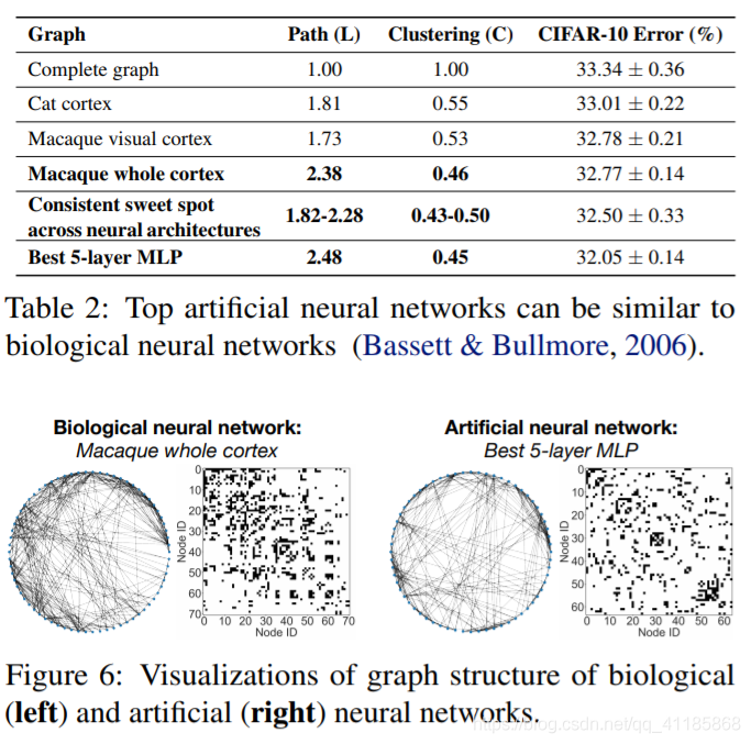
| Network science. The average path length that we measure characterizes how well information is exchanged across the network (Latora & Marchiori, 2001), which aligns with our definition of relational graph that consists of rounds of message exchange. Therefore, the U-shape correlation in Figure 4(b)(d) might indicate a trade-off between message exchange efficiency (Sengupta et al., 2013) and capability of learning distributed representations (Hinton, 1984). Neuroscience. The best-performing relational graph that we discover surprisingly resembles biological neural networks, as is shown in Table 2 and Figure 6. The similarities are in two-fold: (1) the graph measures (L and C) of top artificial neural networks are highly similar to biological neural networks; (2) with the relational graph representation, we can translate biological neural networks to 5-layer MLPs, and found that these networks also outperform the baseline complete graphs. While our findings are preliminary, our approach opens up new possibilities for interdisciplinary research in network science, neuroscience and deep learning. | 网络科学。我们测量的平均路径长度表征了信息在网络中交换的良好程度(Latora & Marchiori, 2001),这与我们对包含轮消息交换的关系图的定义一致。因此,图4(b)(d)中的u形相关性可能表明消息交换效率(Sengupta et al., 2013)和学习分布式表示的能力(Hinton, 1984)之间的权衡。神经科学。我们发现的性能最好的关系图与生物神经网络惊人地相似,如表2和图6所示。相似点有两方面:(1)top人工神经网络的图测度(L和C)与生物神经网络高度相似;(2)利用关系图表示,我们可以将生物神经网络转换为5层MLPs,并发现这些网络的性能也优于基线完整图。虽然我们的发现还处于初步阶段,但我们的方法为网络科学、神经科学和深度学习领域的跨学科研究开辟了新的可能性。 |
6. Related Work
| Neural network connectivity. The design of neural network connectivity patterns has been focused on computational graphs at different granularity: the macro structures, i.e. connectivity across layers (LeCun et al., 1998; Krizhevsky et al., 2012; Simonyan & Zisserman, 2015; Szegedy et al., 2015; He et al., 2016; Huang et al., 2017; Tan & Le, 2019), and the micro structures, i.e. connectivity within a layer (LeCun et al., 1998; Xie et al., 2017; Zhang et al., 2018; Howard et al., 2017; Dao et al., 2019; Alizadeh et al., 2019). Our current exploration focuses on the latter, but the same methodology can be extended to the macro space. Deep Expander Networks (Prabhu et al., 2018) adopt expander graphs to generate bipartite structures. RandWire (Xie et al., 2019) generates macro structures using existing graph generators. However, the statistical relationships between graph structure measures and network predictive performances were not explored in those works. Another related work is Cross-channel Communication Networks (Yang et al., 2019) which aims to encourage the neuron communication through message passing, where only a complete graph structure is considered. |
神经网络的连通性。神经网络连通性模式的设计一直关注于不同粒度的计算图:宏观结构,即跨层连通性(LeCun et al., 1998;Krizhevsky等,2012;Simonyan & Zisserman, 2015;Szegedy等,2015;He et al., 2016;黄等,2017;Tan & Le, 2019)和微观结构,即层内的连通性(LeCun et al., 1998;谢等,2017;张等,2018;Howard等人,2017;Dao等,2019年;Alizadeh等,2019)。我们目前的研究重点是后者,但同样的方法可以扩展到宏观空间。深度扩展器网络(Prabhu et al., 2018)采用扩展器图生成二部图结构。RandWire (Xie等人,2019)使用现有的图生成器生成宏结构。然而,图结构测度与网络预测性能之间的统计关系并没有在这些工作中探索。另一项相关工作是跨通道通信网络(Yang et al., 2019),旨在通过消息传递促进神经元通信,其中只考虑了完整的图结构。 |
| Neural architecture search. Efforts on learning the connectivity patterns at micro (Ahmed & Torresani, 2018; Wortsman et al., 2019; Yang et al., 2018), or macro (Zoph & Le, 2017; Zoph et al., 2018) level mostly focus on improving learning/search algorithms (Liu et al., 2018; Pham et al., 2018; Real et al., 2019; Liu et al., 2019). NAS-Bench101 (Ying et al., 2019) defines a graph search space by enumerating DAGs with constrained sizes (≤ 7 nodes, cf. 64-node graphs in our work). Our work points to a new path: instead of exhaustively searching over all the possible connectivity patterns, certain graph generators and graph measures could define a smooth space where the search cost could be significantly reduced. | 神经结构搜索。在micro学习连接模式的努力(Ahmed & Torresani, 2018;Wortsman等人,2019年;Yang et al., 2018),或macro (Zoph & Le, 2017;Zoph等,2018)水平主要关注于改进学习/搜索算法(Liu等,2018;Pham等人,2018年;Real等人,2019年;Liu等,2019)。NAS-Bench101 (Ying et al., 2019)通过枚举大小受限的DAGs(≤7个节点,我们的工作cf. 64节点图)来定义图搜索空间。我们的工作指向了一个新的路径:不再对所有可能的连通性模式进行穷举搜索,某些图生成器和图度量可以定义一个平滑的空间,在这个空间中搜索成本可以显著降低。 |
7. Discussions
|
Hierarchical graph structure of neural networks. As the first step in this direction, our work focuses on graph structures at the layer level. Neural networks are intrinsically hierarchical graphs (from connectivity of neurons to that of layers, blocks, and networks) which constitute a more complex design space than what is considered in this paper. Extensive exploration in that space will be computationally prohibitive, but we expect our methodology and findings to generalize. Efficient implementation. Our current implementation uses standard CUDA kernels thus relies on weight masking, which leads to worse wall-clock time performance compared with baseline complete graphs. However, the practical adoption of our discoveries is not far-fetched. Complementary to our work, there are ongoing efforts such as block-sparse kernels (Gray et al., 2017) and fast sparse ConvNets (Elsen et al., 2019) which could close the gap between theoretical FLOPS and real-world gains. Our work might also inform the design of new hardware architectures, e.g., biologicallyinspired ones with spike patterns (Pei et al., 2019). |
神经网络的层次图结构。作为这个方向的第一步,我们的工作集中在层层次上的图结构。神经网络本质上是层次图(从神经元的连通性到层、块和网络的连通性),它构成了比本文所考虑的更复杂的设计空间。在那个空间进行广泛的探索在计算上是不可能的,但我们希望我们的方法和发现可以一般化。 高效的实现。我们目前的实现使用标准CUDA内核,因此依赖于weight masking,这导致wall-clock时间性能比基线完整图更差。然而,实际应用我们的发现并不牵强。作为我们工作的补充,还有一些正在进行的工作,如块稀疏核(Gray et al., 2017)和快速稀疏卷积网络(Elsen et al., 2019),它们可以缩小理论失败和现实收获之间的差距。我们的工作也可能为新的硬件架构的设计提供信息,例如,受生物学启发的带有spike图案的架构(Pei et al., 2019)。 |
|
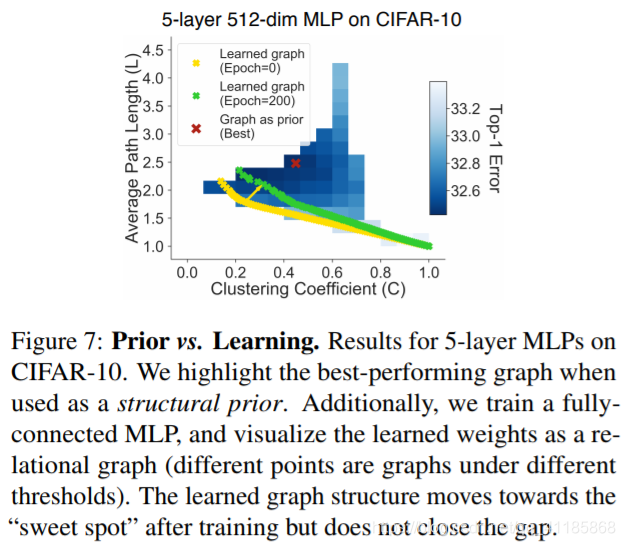
Prior vs. Learning. We currently utilize the relational graph representation as a structural prior, i.e., we hard-wire the graph structure on neural networks throughout training. It has been shown that deep ReLU neural networks can automatically learn sparse representations (Glorot et al., 2011). A further question arises: without imposing graph priors, does any graph structure emerge from training a (fully-connected) neural network?
Figure 7: Prior vs. Learning. Results for 5-layer MLPs on CIFAR-10. We highlight the best-performing graph when used as a structural prior. Additionally, we train a fullyconnected MLP, and visualize the learned weights as a relational graph (different points are graphs under different thresholds). The learned graph structure moves towards the “sweet spot” after training but does not close the gap. |
之前与学习。我们目前利用关系图表示作为结构先验,即。,在整个训练过程中,我们将图形结构硬连接到神经网络上。已有研究表明,深度ReLU神经网络可以自动学习稀疏表示(Glorot et al., 2011)。一个进一步的问题出现了:在不强加图先验的情况下,训练一个(完全连接的)神经网络会产生任何图结构吗?
图7:先验与学习。5层MLPs在CIFAR-10上的结果。当使用结构先验时,我们会突出显示表现最佳的图。此外,我们训练一个完全连接的MLP,并将学习到的权重可视化为一个关系图(不同的点是不同阈值下的图)。学习后的图结构在训练后向“最佳点”移动,但并没有缩小差距。 |
|
As a preliminary exploration, we “reverse-engineer” a trained neural network and study the emerged relational graph structure. Specifically, we train a fully-connected 5-layer MLP on CIFAR-10 (the same setup as in previous experiments). We then try to infer the underlying relational graph structure of the network via the following steps: (1) to get nodes in a relational graph, we stack the weights from all the hidden layers and group them into 64 nodes, following the procedure described in Section 2.2; (2) to get undirected edges, the weights are summed by their transposes; (3) we compute the Frobenius norm of the weights as the edge value; (4) we get a sparse graph structure by binarizing edge values with a certain threshold. We show the extracted graphs under different thresholds in Figure 7. As expected, the extracted graphs at initialization follow the patterns of E-R graphs (Figure 3(left)), since weight matrices are randomly i.i.d. initialized. Interestingly, after training to convergence, the extracted graphs are no longer E-R random graphs and move towards the sweet spot region we found in Section 5. Note that there is still a gap between these learned graphs and the best-performing graph imposed as a structural prior, which might explain why a fully-connected MLP has inferior performance. In our experiments, we also find that there are a few special cases where learning the graph structure can be superior (i.e., when the task is simple and the network capacity is abundant). We provide more discussions in the Appendix. Overall, these results further demonstrate that studying the graph structure of a neural network is crucial for understanding its predictive performance. |
作为初步的探索,我们“逆向工程”一个训练过的神经网络和研究出现的关系图结构。具体来说,我们在CIFAR-10上训练了一个完全连接的5层MLP(与之前的实验相同的设置)。然后尝试通过以下步骤来推断网络的底层关系图结构:(1)为了得到关系图中的节点,我们将所有隐含层的权值进行叠加,并按照2.2节的步骤将其分组为64个节点;(2)对权值的转置求和,得到无向边;(3)计算权值的Frobenius范数作为边缘值;(4)通过对具有一定阈值的边值进行二值化,得到一种稀疏图结构。
我们在图7中显示了在不同阈值下提取的图。正如预期的那样,初始化时提取的图遵循E-R图的模式(图3(左)),因为权重矩阵是随机初始化的。有趣的是,经过收敛训练后,提取的图不再是E-R随机图,而是朝着我们在第5节中发现的最佳点区域移动。请注意,在这些学习图和作为结构先验的最佳性能图之间仍然存在差距,这可能解释了为什么完全连接的MLP性能较差。 在我们的实验中,我们也发现在一些特殊的情况下学习图结构是更好的。当任务简单且网络容量充足时)。我们在附录中提供了更多的讨论。总的来说,这些结果进一步证明了研究神经网络的图结构对于理解其预测性能是至关重要的。
|
|
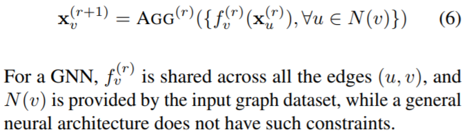
Unified view of Graph Neural Networks (GNNs) and general neural architectures. The way we define neural networks as a message exchange function over graphs is partly inspired by GNNs (Kipf & Welling, 2017; Hamilton et al., 2017; Velickovi ˇ c et al. ´ , 2018). Under the relational graph representation, we point out that GNNs are a special class of general neural architectures where: (1) graph structure is regarded as the input instead of part of the neural architecture; consequently, (2) message functions are shared across all the edges to respect the invariance properties of the input graph. Concretely, recall how we define general neural networks as relational graphs:
Therefore, our work offers a unified view of GNNs and general neural architecture design, which we hope can bridge the two communities and inspire new innovations. On one hand, successful techniques in general neural architectures can be naturally introduced to the design of GNNs, such as separable convolution (Howard et al., 2017), group normalization (Wu & He, 2018) and Squeeze-and-Excitation block (Hu et al., 2018); on the other hand, novel GNN architectures (You et al., 2019b; Chen et al., 2019) beyond the commonly used paradigm (i.e., Equation 6) may inspire more advanced neural architecture designs. |
图形神经网络(GNNs)和一般神经结构的统一视图。我们将神经网络定义为图形上的信息交换功能的方式,部分受到了gnn的启发(Kipf & Welling, 2017;Hamilton等,2017;Velickoviˇc et al .´, 2018)。在关系图表示下,我们指出gnn是一类特殊的一般神经结构,其中:(1)将图结构作为输入,而不是神经结构的一部分;因此,(2)消息函数在所有边之间共享,以尊重输入图的不变性。具体地说,回想一下我们是如何将一般的神经网络定义为关系图的: 因此,我们的工作提供了一个关于gnn和一般神经结构设计的统一观点,我们希望能够搭建这两个社区的桥梁,激发新的创新。一方面,一般神经结构中的成功技术可以自然地引入到gnn的设计中,如可分离卷积(Howard et al., 2017)、群归一化(Wu & He, 2018)和挤压-激励块(Hu et al., 2018);另一方面,新的GNN架构(You et al., 2019b;陈等人,2019)超越了常用的范式(即,(6)可以启发更先进的神经结构设计。 |
8. Conclusion
| In sum, we propose a new perspective of using relational graph representation for analyzing and understanding neural networks. Our work suggests a new transition from studying conventional computation architecture to studying graph structure of neural networks. We show that well-established graph techniques and methodologies offered in other science disciplines (network science, neuroscience, etc.) could contribute to understanding and designing deep neural networks. We believe this could be a fruitful avenue of future research that tackles more complex situations. |
最后,我们提出了一种利用关系图表示来分析和理解神经网络的新观点。我们的工作提出了一个新的过渡,从研究传统的计算结构到研究神经网络的图结构。我们表明,在其他科学学科(网络科学、神经科学等)中提供的成熟的图形技术和方法可以有助于理解和设计深度神经网络。我们相信这将是未来解决更复杂情况的研究的一个富有成效的途径。 |
Acknowledgments
| This work is done during Jiaxuan You’s internship at Facebook AI Research. Jure Leskovec is a Chan Zuckerberg Biohub investigator. The authors thank Alexander Kirillov, Ross Girshick, Jonathan Gomes Selman, Pan Li for their helpful discussions. | 这项工作是在You Jiaxuan在Facebook AI Research实习期间完成的。Jure Leskovec是陈-扎克伯格生物中心的调查员。作者感谢Alexander Kirillov, Ross Girshick, Jonathan Gomes Selman和Pan Li的讨论。 |

- 《Graph Neural Networks: A Review of Methods and Applications》阅读笔记
- Advanced Applications of Neural Networks and Artificial Intelligence: A Review
- Paper:《Generating Sequences With Recurrent Neural Networks》的翻译和解读
- 《mastering the game of GO wtth deep neural networks and tree search》研究解读
- Paper:《YOLOv4: Optimal Speed and Accuracy of Object Detection》的翻译与解读
- 深入解读AlphaGo,Nature-2016:Mastering the game of Go with deep neural networks and tree search
- Mastering the game of Go with deep neural networks and tree search 概括
- Intriguing properties of neural networks手动翻译
- 学习摘要:Methods for interpreting and understanding deep neural networks
- Quantization and Training of Neural Networks for Efficient Integer-Arithmetic-Only Inference
- Bridging Collaborative Filtering and Semi-Supervised Learning:paper翻译与解读
- RNN(2) ------ “《A Critical Review of Recurrent Neural Networks for Sequence Learning》RNN综述性论文讲解”(转载)
- 论文笔记之Label-Free Supervision of Neural Networks with Physics and Domain Knowledge
- End-to-End Learning of Deformable Mixture of Parts and Deep Convolutional Neural Networks for Human
- 论文笔记:Mastering the game of Go with deep neural networks and tree search
- paper 157:文章解读--How far are we from solving the 2D & 3D Face Alignment problem?-(and a dataset of 230,000 3D facial landmarks)
- deeplearning论文学习笔记(2)A critical review of recurrent neural networks for sequence learning
- 《On Classification of Distorted Images with Deep Convolutional Neural Networks》翻译
- A Java Library of Graph Algorithms and Optimization (Discrete Mathematics and Its Applications)
- Highly Efficient Forward and Backward Propagation of Convolutional Neural Networks for Pixelwise Cla