手写汉字数字识别（构建数据集+CNN神经网络）

期末，P老师布置了一个大作业，自己构建数据集实现手写汉字数字的识别。太捞了，记录一下过程。大概花了一个下午加半个晚上，主要是做数据集花时间。

一、构建数据集——使用h5py

1.收集数据，这部分由我勤劳的室友们一起手写了800个汉字 一、二、三、四、五、六、七、八、九、十完成。这部分也没啥好说的，慢慢写呗。我们用了IPAD，然后截图，这样出来的图片质量比较好。
2.对图像进行处理。将图像转化为(64,64,3)的矩阵，对图像批量编号及分类。这里新建了一个py文件，代码如下。

import h5py
import os
import numpy as np
from PIL import Image
import tensorflow as tf
import matplotlib.pyplot as plt
import sklearn
from sklearn import preprocessing
import scipy

#未处理图片位置
orig_picture = r'C:\Users\10595\Desktop\dataset\image'

#已处理图片存储位置
gen_picturn = r'C:\Users\10595\Desktop\dataset\data'

#查询需要分类的类别以及总样本个数
classes = ["one","two","three","four","five","six","seven","eight","nine","ten"]

def get_traindata(orig_dir,gen_dir,classes):
i = 0
for index,name in enumerate(classes):
class_path = orig_dir + '\\' + name + '\\' #扫描原始图片
gen_train_path = gen_dir +'\\' + name   #判断是否有文件夹
folder = os.path.exists(gen_train_path)
if not folder :
os.makedirs(gen_train_path)
print(gen_train_path,'new file')
else:
print('There is this flie')
#给图片加编号保存
for imagename_dir in os.listdir(class_path):
i += 1
origimage_path = class_path + imagename_dir
#统一格式
image_data = Image.open(origimage_path).convert('RGB')
image_data = image_data.resize((64,64))
image_data.save(gen_train_path + '\\' + name + str(i) + '.jpg' )
num_samples = i
print('picturn ：%d' % num_samples)

if __name__ == '__main__':
get_traindata(orig_picture,gen_picturn,classes)

3.使用h5py将图像打包成数据集

import os
import numpy as np
from PIL import Image
import h5py
import scipy
import matplotlib.pyplot as plt
#搞了十个我也很困惑，不知道有什么简便方法
one = []
label_one = []
two = []
label_two = []
three = []
label_three = []
four = []
label_four = []
five = []
label_five = []
six = []
label_six = []
seven = []
label_seven = []
eight = []
label_eight = []
nine = []
label_nine = []
ten = []
label_ten = []

def get_files(file_dir):
for file in os.listdir(file_dir + '\\' + 'one'):
one.append(file_dir +'\\'+'one'+'\\'+ file)
label_one.append(0)
for file in os.listdir(file_dir + '\\' + 'two'):
two.append(file_dir +'\\'+'two'+'\\'+ file)
label_two.append(1)
for file in os.listdir(file_dir + '\\' + 'three'):
three.append(file_dir +'\\'+'three'+'\\'+ file)
label_three.append(2)
for file in os.listdir(file_dir + '\\' + 'four'):
four.append(file_dir +'\\'+'four'+'\\'+ file)
label_four.append(3)
for file in os.listdir(file_dir + '\\' + 'five'):
five.append(file_dir +'\\'+'five'+'\\'+ file)
label_five.append(4)
for file in os.listdir(file_dir + '\\' + 'six'):
six.append(file_dir +'\\'+'six'+'\\'+ file)
label_six.append(5)
for file in os.listdir(file_dir + '\\' + 'seven'):
seven.append(file_dir +'\\'+'seven'+'\\'+ file)
label_seven.append(6)
for file in os.listdir(file_dir + '\\' + 'eight'):
eight.append(file_dir +'\\'+'eight'+'\\'+ file)
label_eight.append(7)
for file in os.listdir(file_dir + '\\' + 'nine'):
nine.append(file_dir +'\\'+'nine'+'\\'+ file)
label_nine.append(8)
for file in os.listdir(file_dir + '\\' + 'ten'):
ten.append(file_dir +'\\'+'ten'+'\\'+ file)
label_ten.append(9)
#把所有数据集进行合并
image_list = np.hstack((one,two,three,four,five,six,seven,eight,nine,ten))
label_list = np.hstack((label_one,label_two,label_three,label_four,label_five,label_six,label_seven,label_eight,label_nine,label_ten))

#利用shuffle打乱顺序
temp = np.array([image_list, label_list])
temp = temp.transpose()
np.random.shuffle(temp)

#从打乱的temp中再取出list（img和lab）
image_list = list(temp[:, 0])
label_list = list(temp[:, 1])
label_list = [int(i) for i in label_list]

return image_list,label_list
train_dir = r'C:\Users\10595\Desktop\dataset\data'
image_list,label_list = get_files(train_dir)
Train_image =  np.random.rand(len(image_list)-50, 64, 64, 3).astype('float32')
#这里50为测试集，根据需求改
Train_label = np.random.rand(len(image_list)-50, 1).astype('int')

Test_image =  np.random.rand(50, 64, 64, 3).astype('float32')
Test_label = np.random.rand(50, 1).astype('int')
for i in range(len(image_list)-50):
Train_image[i] = np.array(plt.imread(image_list[i]))
Train_label[i] = np.array(label_list[i])

for i in range(len(image_list)-50, len(image_list)):
Test_image[i+50-len(image_list)] = np.array(plt.imread(image_list[i]))
Test_label[i+50-len(image_list)] = np.array(label_list[i])

f = h5py.File('data.h5', 'w')
f.create_dataset('X_train', data=Train_image)
f.create_dataset('y_train', data=Train_label)
f.create_dataset('X_test', data=Test_image)
f.create_dataset('y_test', data=Test_label)
f.close()
#文件生成在此py文件同一文件夹下

这样我们就得到了一个.h文件，里面存放着我们的图片信息。

二、使用CNN进行训练预测

以下均是在Jupyter Notebook 中实现滴~

import math
import numpy as np
import h5py
import matplotlib.pyplot as plt
import scipy
from PIL import Image
from scipy import ndimage
import tensorflow as tf
from tensorflow.python.framework import ops
from cnn_utils import *
#载入我们刚才制作的h5数据集
train_dataset = h5py.File('data.h5', 'r')
X_train_orig = np.array(train_dataset['X_train'][:])
Y_train_orig = np.array(train_dataset['y_train'][:])
X_test_orig = np.array(train_dataset['X_test'][:])
Y_test_orig = np.array(train_dataset['y_test'][:])
X_train = X_train_orig/255.
X_test = X_test_orig/255.#归一化

让我们来康康我们做的数据集长得怎么样

t = 5
plt.imshow(X_train[t])
print("y = "+str(np.squeeze(Y_train_orig[t])+1))

#确认一下数据集的大小
Y_train_orig = Y_train_orig.T
Y_test_orig = Y_test_orig.T
Y_train = convert_to_one_hot(Y_train_orig, 10).T
Y_test = convert_to_one_hot(Y_test_orig, 10).T
print ("number of training examples = " + str(X_train.shape[0]))
print ("number of test examples = " + str(X_test.shape[0]))
print ("X_train shape: " + str(X_train.shape))
print ("Y_train shape: " + str(Y_train.shape))
print ("X_test shape: " + str(X_test.shape))
print ("Y_test shape: " + str(Y_test.shape))
conv_layers = {}
print(Y_train[5])

#开始Tensorflow
def create_placeholders(n_H0, n_W0, n_C0, n_y):
X = tf.placeholder(tf.float32, shape=[None, n_H0, n_W0, n_C0])
Y = tf.placeholder(tf.float32, shape=[None, n_y])
return X, Y
X, Y = create_placeholders(64, 64, 3, 10)
print ("X = " + str(X))
print ("Y = " + str(Y))
def initialize_parameters():
tf.set_random_seed(1)                              # so that your "random" numbers match ours

W1 = tf.get_variable("W1",  [4, 4, 3, 8], initializer=tf.contrib.layers.xavier_initializer(seed=0))
W2 = tf.get_variable("W2",  [2, 2, 8, 16], initializer=tf.contrib.layers.xavier_initializer(seed=0))
W3 = tf.get_variable("W3",  [64,10], initializer=tf.contrib.layers.xavier_initializer(seed=0))

parameters = {"W1": W1,
"W2": W2,
"W3": W3}

return parameters

tf.reset_default_graph()
with tf.Session() as sess_test:
parameters = initialize_parameters()
init = tf.global_variables_initializer()
sess_test.run(init)
print("W1 = " + str(parameters["W1"].eval()[1,1,1]))
print("W2 = " + str(parameters["W2"].eval()[1,1,1]))
print("W3 = " + str(parameters["W3"].eval()[1,1]))

def forward_propagation(X, parameters):
# Retrieve the parameters from the dictionary "parameters"
W1 = parameters['W1']
W2 = parameters['W2']
W3 = parameters['W3']
# CONV2D: stride of 1, padding 'SAME'
Z1 = tf.nn.conv2d(X, W1, strides=[1,1,1,1], padding="SAME")
# RELU
A1 = tf.nn.relu(Z1)
# MAXPOOL: window 8x8, sride 8, padding 'SAME'
P1 = tf.nn.max_pool(A1, ksize=[1,8,8,1], strides=[1,8,8,1], padding="SAME")
# CONV2D: filters W2, stride 1, padding 'SAME'
Z2 = tf.nn.conv2d(P1, W2, strides=[1,1,1,1], padding="SAME")
# RELU
A2 = tf.nn.relu(Z2)
# MAXPOOL: window 4x4, stride 4, padding 'SAME'
P2 = tf.nn.max_pool(A2, ksize=[1,4,4,1], strides=[1,4,4,1], padding="SAME")
# FLATTEN
P2 = tf.contrib.layers.flatten(P2)
print(P2.shape)
# FULLY-CONNECTED without non-linear activation function (not not call softmax).
# 6 neurons in output layer. Hint: one of the arguments should be "activation_fn=None"
Z3 = tf.matmul(P2, W3)
#tf.contrib.layers.fully_connected(P2, 6, activation_fn=None, weights_initializer=tf.contrib.layers.xavier_initializer(seed=0))
return Z3

tf.reset_default_graph()

with tf.Session() as sess:
np.random.seed(1)
X, Y = create_placeholders(64, 64, 3, 10)
parameters = initialize_parameters()
Z3 = forward_propagation(X, parameters)
init = tf.global_variables_initializer()
sess.run(init)
a = sess.run(Z3, {X: np.random.randn(2,64,64,3), Y: np.random.randn(2,10)})
print("Z3 = " + str(a))

# GRADED FUNCTION: compute_cost
def compute_cost(Z3, Y):
cost = tf.nn.softmax_cross_entropy_with_logits(logits = Z3, labels = Y)
cost = tf.reduce_mean(cost)
return cost

tf.reset_default_graph()

with tf.Session() as sess:
np.random.seed(1)
X, Y = create_placeholders(64, 64, 3, 10)
parameters = initialize_parameters()
Z3 = forward_propagation(X, parameters)
cost = compute_cost(Z3, Y)
init = tf.global_variables_initializer()
sess.run(init)
a = sess.run(cost, {X: np.random.randn(4,64,64,3), Y: np.random.randn(4,10)})
print("cost = " + str(a))

def model(X_train, Y_train, X_test, Y_test, learning_rate = 0.009,
num_epochs = 100, minibatch_size = 64, print_cost = True):

ops.reset_default_graph()                         # to be able to rerun the model without overwriting tf variables
tf.set_random_seed(1)                             # to keep results consistent (tensorflow seed)
seed = 3                                          # to keep results consistent (numpy seed)
(m, n_H0, n_W0, n_C0) = X_train.shape
n_y = Y_train.shape[1]
costs = []                                        # To keep track of the cost

X, Y = create_placeholders(n_H0, n_W0, n_C0, n_y)

parameters = initialize_parameters()

# Forward propagation: Build the forward propagation in the tensorflow graph
Z3 = forward_propagation(X, parameters)

# Cost function: Add cost function to tensorflow graph
cost = compute_cost(Z3, Y)

# Backpropagation: Define the tensorflow optimizer. Use an AdamOptimizer that minimizes the cost.
optimizer = tf.train.AdamOptimizer(learning_rate=learning_rate).minimize(cost)

# Initialize all the variables globally
init = tf.global_variables_initializer()

saver = tf.train.Saver()
# Start the session to compute the tensorflow graph
with tf.Session() as sess:

# Run the initialization
sess.run(init)

# Do the training loop
for epoch in range(num_epochs):

minibatch_cost = 0.
num_minibatches = int(m / minibatch_size) # number of minibatches of size minibatch_size in the train set
seed = seed + 1
minibatches = random_mini_batches(X_train, Y_train, minibatch_size, seed)

for minibatch in minibatches:

# Select a minibatch
(minibatch_X, minibatch_Y) = minibatch
# IMPORTANT: The line that runs the graph on a minibatch.
# Run the session to execute the optimizer and the cost, the feedict should contain a minibatch for (X,Y).
_ , temp_cost = sess.run([optimizer, cost], feed_dict={X: minibatch_X, Y: minibatch_Y})

minibatch_cost += temp_cost / num_minibatches

# Print the cost every epoch
if print_cost == True and epoch % 5 == 0:
print ("Cost after epoch %i: %f" % (epoch, minibatch_cost))
if print_cost == True and epoch % 1 == 0:
costs.append(minibatch_cost)
# save parameters
if epoch == num_epochs-1:
saver.save(sess,'params.ckpt')

# plot the cost
plt.plot(np.squeeze(costs))
plt.ylabel('cost')
plt.xlabel('iterations (per tens)')
plt.title("Learning rate =" + str(learning_rate))
plt.show()

# Calculate the correct predictions
predict_op = tf.argmax(Z3, 1)
correct_prediction = tf.equal(predict_op, tf.argmax(Y, 1))

# Calculate accuracy on the test set
accuracy = tf.reduce_mean(tf.cast(correct_prediction, "float"))
print(accuracy)
train_accuracy = accuracy.eval({X: X_train, Y: Y_train})
test_accuracy = accuracy.eval({X: X_test, Y: Y_test})
print("Train Accuracy:", train_accuracy)
print("Test Accuracy:", test_accuracy)

return train_accuracy, test_accuracy, parameters

#终于开始训练啦~
_, _, parameters = model(X_train, Y_train, X_test, Y_test)

学习结果如下图所示：（训练集精确度竟然轻松达到了1.0，显然我们的数据集有、、糟糕）测试精度非常高，0.98！可以交作业了！

三、来测试一下吧

1.先来试试训练集里的图片

index = np.random.randint(0,745) # choose from trainset randomly
print(index)
tf.reset_default_graph()

#predict
with tf.Session() as sess:
np.random.seed(1)
X, Y = create_placeholders(64, 64, 3, 10)
parameters = initialize_parameters()

# initial parameters
init = tf.global_variables_initializer()
sess.run(init)

# restore parameters
variables = tf.global_variables()
saver = tf.train.Saver()
saver.restore(sess,'params.ckpt')

# predict
parametses = {variables[0],variables[1],variables[2]}
predict_result = forward_propagation(X, parameters)

#prepare data, use normalized data
X_from_trainset = X_train[index].astype(np.float32)
X_from_trainset = np.reshape(X_from_trainset,[1,64,64,3])
Y_from_trainset = Y_train[index]
Y_from_trainset = np.reshape(Y_from_trainset,[1,10])

# display this picture
plt.imshow(X_train_orig[index]/255)
print ("y = " + str(np.squeeze(Y_train_orig[:,index])+1))
#

# display predict result
a = sess.run(predict_result, {X: X_from_trainset, Y: Y_from_trainset})
print(a)
predict_class = np.argmax(a, 1)
print("predict y = " + str(np.squeeze(predict_class)+1))

得到如下结果：

2.再来试试测试集

#np.random.seed(1)
tf.reset_default_graph()
index = np.random.randint(0,50) # choose from testset randomly
print(index)
#predict
with tf.Session() as sess:

X, Y = create_placeholders(64, 64, 3, 10)
parameters = initialize_parameters()

# initial parameters
init = tf.global_variables_initializer()
sess.run(init)

# restore parameters
variables = tf.global_variables()
saver = tf.train.Saver()
saver.restore(sess,'params.ckpt')

#predict
parametses = {variables[0],variables[1],variables[2]}
predict_result = forward_propagation(X, parameters)

#prepare data, use nomalized data
X_from_testset = X_test[index].astype(np.float32)
X_from_testset = np.reshape(X_from_testset,[1,64,64,3])
Y_from_testset = Y_test[index]
Y_from_testset = np.reshape(Y_from_testset,[1,10])
#X,Y = create_placeholders(64, 64, 3, 10)

# display this picture
plt.imshow(X_test_orig[index]/255)
print ("y = " + str(np.squeeze(Y_test_orig[:,index])+1))
#

#display predict result
a = sess.run(predict_result, {X: X_from_testset, Y: Y_from_testset})
print(a)
predict_class = np.argmax(a, 1)
print("predict y = " + str(np.squeeze(predict_class)+1))

结果如下图：（不得不说我室友的字是真的丑蛤蛤）

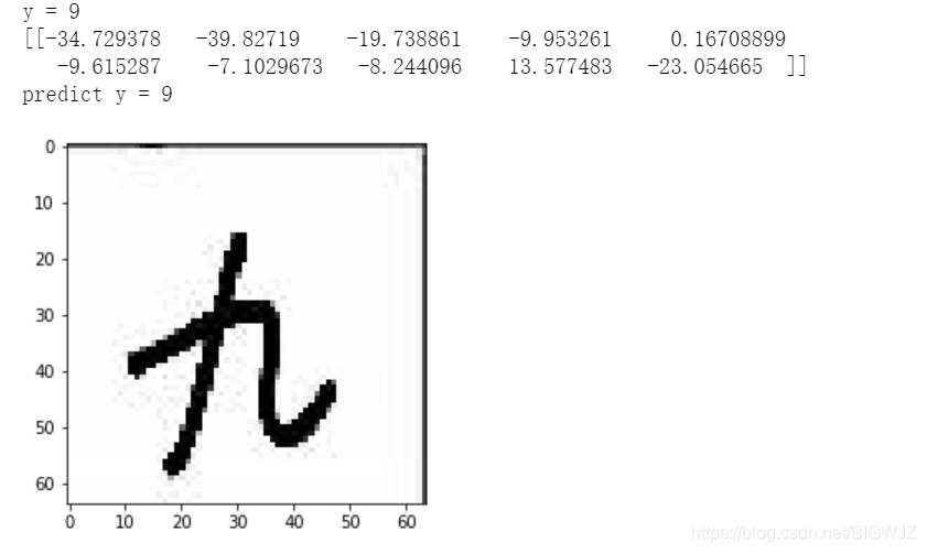
3.最后，来试一张不存在与数据集中的新图片，没错，是我手写的

tf.reset_default_graph()

#这个图片名字叫做test.jpg
my_image = Image.open('test.jpg')
my_image = my_image.resize((64,64))
# display this picture
plt.imshow(my_image)

#prepare data
X_my_image = np.array(my_image)/255. # normalization
X_my_image = X_my_image.astype(np.float32)
X_my_image = np.reshape(X_my_image,[1,64,64,3])

with tf.Session() as sess:
np.random.seed(1)
X, Y = create_placeholders(64, 64, 3, 10)
parameters = initialize_parameters()

#initialize parameters
init = tf.global_variables_initializer()
sess.run(init)

#restore parameters
variables = tf.global_variables()
saver = tf.train.Saver()
saver.restore(sess,'params.ckpt')

#predict
parametses = {variables[0],variables[1],variables[2]}
predict_result = forward_propagation(X, parameters)

#display predict result
a = sess.run(predict_result, {X: X_my_image, Y: [[1,0,0,0,0,0,0,0,0,0]]})
print(a)
predict_class = np.argmax(a, 1)
print("predict y = " + str(predict_class+1))

结果当然是预测成功啦：

附：CNN_utils 如下

import math
import numpy as np
import h5py
import matplotlib.pyplot as plt
import tensorflow as tf
from tensorflow.python.framework import ops

def random_mini_batches(X, Y, mini_batch_size = 64, seed = 0):

m = X.shape[0]                  # number of training examples
mini_batches = []
np.random.seed(seed)

# Step 1: Shuffle (X, Y)
permutation = list(np.random.permutation(m))
shuffled_X = X[permutation,:,:,:]
shuffled_Y = Y[permutation,:]

# Step 2: Partition (shuffled_X, shuffled_Y). Minus the end case.
num_complete_minibatches = math.floor(m/mini_batch_size) # number of mini batches of size mini_batch_size in your partitionning
for k in range(0, num_complete_minibatches):
mini_batch_X = shuffled_X[k * mini_batch_size : k * mini_batch_size + mini_batch_size,:,:,:]
mini_batch_Y = shuffled_Y[k * mini_batch_size : k * mini_batch_size + mini_batch_size,:]
mini_batch = (mini_batch_X, mini_batch_Y)
mini_batches.append(mini_batch)

# Handling the end case (last mini-batch < mini_batch_size)
if m % mini_batch_size != 0:
mini_batch_X = shuffled_X[num_complete_minibatches * mini_batch_size : m,:,:,:]
mini_batch_Y = shuffled_Y[num_complete_minibatches * mini_batch_size : m,:]
mini_batch = (mini_batch_X, mini_batch_Y)
mini_batches.append(mini_batch)

return mini_batches

def convert_to_one_hot(Y, C):
Y = np.eye(C)[Y.reshape(-1)].T
return Y

def forward_propagation_for_predict(X, parameters):

# Retrieve the parameters from the dictionary "parameters"
W1 = parameters['W1']
b1 = parameters['b1']
W2 = parameters['W2']
b2 = parameters['b2']
W3 = parameters['W3']
b3 = parameters['b3']
# Numpy Equivalents:
Z1 = tf.add(tf.matmul(W1, X), b1)                      # Z1 = np.dot(W1, X) + b1
A1 = tf.nn.relu(Z1)                                    # A1 = relu(Z1)
Z2 = tf.add(tf.matmul(W2, A1), b2)                     # Z2 = np.dot(W2, a1) + b2
A2 = tf.nn.relu(Z2)                                    # A2 = relu(Z2)
Z3 = tf.add(tf.matmul(W3, A2), b3)                     # Z3 = np.dot(W3,Z2) + b3

return Z3

def predict(X, parameters):

W1 = tf.convert_to_tensor(parameters["W1"])
b1 = tf.convert_to_tensor(parameters["b1"])
W2 = tf.convert_to_tensor(parameters["W2"])
b2 = tf.convert_to_tensor(parameters["b2"])
W3 = tf.convert_to_tensor(parameters["W3"])
b3 = tf.convert_to_tensor(parameters["b3"])

params = {"W1": W1,
"b1": b1,
"W2": W2,
"b2": b2,
"W3": W3,
"b3": b3}

x = tf.placeholder("float", [12288, 1])

z3 = forward_propagation_for_predict(x, params)
p = tf.argmax(z3)

sess = tf.Session()
prediction = sess.run(p, feed_dict = {x: X})

return prediction