机器学习中随机森林、神经网络和xgboost的分类问题和判断分布的方法

一、

最近在做机器学习分类问题的评价，写了一些代码和评价方法

总的来说，用随机森林和其他分类器做好分类后对混淆矩阵进行处理可以得到rr和kappa系数，此外对于二分类变量，还可以计算出roc曲线和auc面积，在对随机森林的计算中，我得到了以下的代码：

library(randomForest)

library(moments)

library(car)

library("soiltexture")

library(caret)

setwd("d:/Z/test")

A<-matrix(0,30,1)

ALOW<-matrix(0,30,1)

AUP<-matrix(0,30,1)

KAPPA<-matrix(0,30,1)

trainall=read.csv("classT.csv")

trainall$veget <-as.factor(trainall$veget)

trainall$soilt <-as.factor(trainall$soilt)

trainall$lc <- as.factor(trainall$lc)

trainall$lcc<- as.factor(trainall$lcc)

trainall$geo <- as.factor(trainall$geo)

for (ttt in 1:30)

{

while(TRUE)

{

while(TRUE)

{

index<- sample(1:nrow(trainall), 449)

train<- trainall[index, ]

testdata<- trainall[-index, ]

train$class<- factor(train$class)

testdata$class<- factor(testdata$class)

if(length(levels(train$class))==10&&length(levels(testdata$class))==10)

break

}

TF=randomForest(class~.,data=train,mtry=5,ntree=1000,importance=T)

pre<-predict(TF,testdata,tpye=prob)

if(length(levels(pre))==10)

break

}

cc<-confusionMatrix(pre,testdata$class)

##cc$overall

a<-matrix(cc$overall)

A[ttt]=a[1,1]

KAPPA[ttt]=a[2,1]

ALOW[ttt]=a[3,1]

AUP[ttt]=a[4,1]

}

a1<-0

a2<-0

a3<-0

a4<-0

for(eee in 1:30)

{

 a1<-a1+A[eee]

 a2<-a2+KAPPA[eee]

 a3<-a3+ALOW[eee]

 a4<-a4+AUP[eee]

}

RESULT<-matrix(0,4,2)

RESULT[1,1]="Accuracy "

RESULT[2,1]="Kappa"

RESULT[3,1]="AccuracyLower"

RESULT[4,1]="AccuracyUpper"

RESULT[1,2]=a1/30

RESULT[2,2]=a2/30

RESULT[3,2]=a3/30

RESULT[4,2]=a4/30

write.table(RESULT, file ="d:/Z/test/RESULT1.txt", row.names = F, quote = F)

可以做30次交叉验证得出rr和kappa系数，但是最后结果得到的是直接的因子型变量，并不是我们要计算roc曲线而需要的prob，所以这种情况下不能得到roc曲线的计算，只用正确分类精度和混淆矩阵的kappa系数来评价分类器的好坏即可，在一些二分类变量中，我们计算出一些概率分布，我们可以通过r中以下的代码完成对roc和auc的计算：

library(pROC)

modelroc <- roc(newdata$y,pre)

plot(modelroc, print.auc=TRUE,auc.polygon=TRUE, grid=c(0.1, 0.2),

    grid.col=c("green", "red"), max.auc.polygon=TRUE,

    auc.polygon.col="skyblue", print.thres=TRUE)

######################

library(ROCR)

pred <- prediction(pre,newdata$y)

performance(pred,'auc')@y.values #AUC值

perf <- performance(pred,'tpr','fpr')

plot(perf)

###########

roc(myData$label, myData$score, plot=TRUE,print.thres=TRUE, print.auc=TRUE) 

###############

roc1 <- roc(myData$label, myData$score)

roc2 <- roc(myData2$label,myData2$score)

plot(roc1, col="blue")

plot.roc(roc2, add=TRUE,col="red")

具体方法参考cran pROC

二、在对xgboost的分类问题中遇到了一些问题，

library(xgboost)

library(moments)

library(car)

library(sp)

library("soiltexture")

setwd("d:/Z/test")

trainall=read.csv("classTF.csv")

trainall=read.csv("classT.csv")

index<- sample(1:nrow(trainall), 449)

train<- trainall[index, ]

testdata<- trainall[-index, ]

##############data.matrix(X_test[,-1]))

ttt<-as.matrix(train)

tt<-as.matrix(testdata)

TF=xgboost(data=ttt[,-19],label=train$sand,max.depth= 2, eta = 1, nthread = 2, nround = 2, objective = "binary:logistic")

TF=xgboost(data=ttt[,-19],label=train$sand,max.depth= 10, eta = 1, nthread = 2, nround = 10)

TF=xgboost(data=ttt[,-19],label=train$sand,max.depth= 10, subsample=1,colsample_bytree=0.8,,min_child_weight=0.8,eta = 1, nthread =2, nround = 10)

#######TF=xgboost(data=ttt[,-19],label=train$sand,max.depth= 10, subsample=1,min_child_weight=0.8,colsample_bytree=0.8,eta = 1, nthread =2, nround = 10)

TF=xgboost(data=ttt,label=train$sand,max.depth= 2, eta = 1, nthread = 2, nround = 2)

importance_matrix <- xgb.importance(TF)

TF=xgboost(data=ttt[,-19],label=train$sand,max.depth= 5, eta = 1, nthread = 2, nround = 2)

pre<-predict(TF,tt[,-19])

 apre<-as.matrix(pre)

att<-as.matrix(testdata$sand)

c<-cbind(apre,att)

mse<-0

for(i in 1:193)

 {

   mse<-mse+(att[i]-apre[i])*(att[i]-apre[i])

 }

sqrt(mse/193)

rr1<-0

rr2<-0

rr3<-0

 for(i in 1:193)

 {

   rr1<-rr1+att[i]

 }

rr1<-rr1/193

 for(j in 1:193)

 {

   rr2<-rr2+(apre[j]-att[j])*(apre[j]-att[j])

 }

 for(k in 1:193)

 {

   rr3<-rr3+(att[k]-rr1)*(att[k]-rr1)

 }

 RR<-(1-rr2/rr3)*100

经过此代码的结果并没有提高的很多，反而会有一些下降，主题是参数的调整问题，还有就是数据在这个算法的放置问题，不知道是不是与随机森林的不同（rf），迭代的次数没有设置好，问题与神经网络类似，得到的预测数值有很多重复值。这是一个不好的预测，表明了环境变量没有很好的应用在这个模型上。对于出图的程序也存在这个问题。

接下来将对xgboost的参数和变量的加入进行一些变化的调整，与rf包和ranger包进行对比。

三、

对于glm的回归预测模型，效果不好的原因（40%rr，16rmse）

library(xgboost)

library(moments)

library(car)library(sp)

library("soiltexture")

library(stats)

setwd("d:/Z/test")

RMSE<-matrix(0,30,1)

RR<-matrix(0,30,1)

for(ii in 1:30)

{

trainall=read.csv("train642.csv")

index<- sample(1:nrow(trainall), 449)

train<- trainall[index, ]

t2<- trainall[-index, ]

TF1<-glm(ILR_1~veget+geo+soilt+lc+aspect+slope+curvature+rain+tem+dem+soc+ndvi+conindex+lon+lat+plan+profile+vellyd+bi+savi+rain1,data=train,family=gaussian())

TF2<-glm(ILR_2~veget+geo+soilt+lc+aspect+slope+curvature+rain+tem+dem+soc+ndvi+conindex+lon+lat+plan+profile+vellyd+bi+savi+rain1,data=train,family=gaussian())

ILR_1.pre<-predict(TF1,t2)

ILR_2.pre<-predict(TF2,t2)

RF.prediction<-matrix(0,193,2)

RF.prediction[,1]<-ILR_1.pre

RF.prediction[,2]<-ILR_2.pre

pred.Sand =100/(1+exp(sqrt(2)*RF.prediction[,1])+sqrt(exp(sqrt(2)*RF.prediction[,1]))*exp(sqrt(3/2)*RF.prediction[,2]))

apre<-as.matrix(pred.Sand)

att<-as.matrix(t2$sand)

c<-cbind(apre,att)

mse<-0

for(i in 1:193)

 {

   mse<-mse+(att[i]-apre[i])*(att[i]-apre[i])

 }

RMSE[ii]<-sqrt(mse/193)

rr1<-0

rr2<-0

rr3<-0

 for(i in 1:193)

 {

   rr1<-rr1+att[i]

 }

rr1<-rr1/193

 for(j in 1:193)

 {

   rr2<-rr2+(apre[j]-att[j])*(apre[j]-att[j])

 }

 for(k in 1:193)

 {

   rr3<-rr3+(att[k]-rr1)*(att[k]-rr1)

 }

 RR[ii]<-(1-rr2/rr3)*100

 ii<ii+1

}

RR

RMSE

rrr<-0

rmsee<-0

for(i in 1:30)

{

  rrr<-rrr+RR[i]

  rmsee<-rmsee+RMSE[i]

}

rr<-rrr/30

rmse<-rmsee/30

对于以上的程序中，我得到了rr和rmse的值，分别为40%和16

与回归的rf相比，这是不好的（50%，14），我们注意到在公式中的glm选择的方法为高斯，即需要样本符合正态分布才可以，但是我们通过这样的一个r语言包：

library(fitdistrplus)

可以得到一个未知分布的分布情况，并根据最小的误差选择出最符合这个数据的分布。

x <- rnorm(642)

这是一个正态分布的数据，我们可以容易的看出这个程序给出的最接近分布。

但是我们的数据在整个流域中并不是一个正态分布

此外的两种检验方法：

1.

sand<-train$sand

ilr<-train$ILR_1

x <- rnorm(642)

x2 <- rnorm(642)

ks.test(x, x2)

ks.test(x, 'pnorm')

ks.test(ilr, 'pnorm')

ks.test(sand, 'pnorm')

ks.test(x, 'pexp')

2.

x <- rnorm(642)

x2 <- rnorm(642)

shapiro.test(x2)

chisq.test(sand)

回到我们的数据问题，我们又原始数据sand’和对数转化数据两种，我们分别对他们的数据分布类型做图：

Sand：

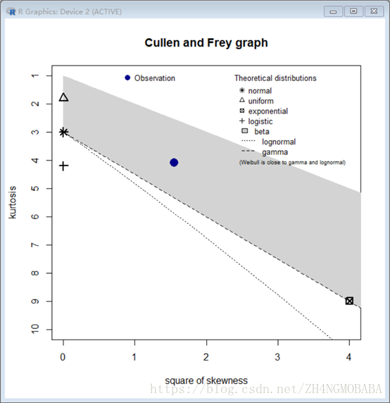
统计为：

min: 0.98   max:  99.66

median: 25.06398

mean: 30.57073

estimated sd:  21.96976

estimated skewness:  1.246292

estimated kurtosis:  4.079616

Ilr为：

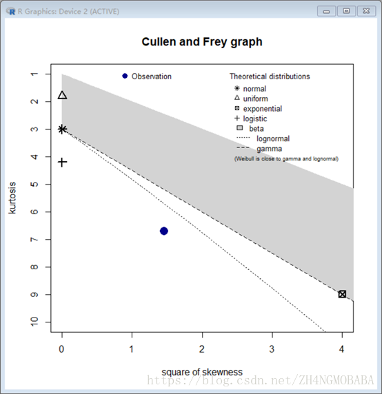
统计为;

min: -4.506902   max:  2.968629

median: 0.6145865

mean: 0.5308409

estimated sd:  0.924625

estimated skewness:  -1.206198

estimated kurtosis:  6.71577

我们可以看到我们的数据sand应该是gamma或者beta分布的

Ilr应该是对数正态分布，而不是正态分布