tensorflow 核心流程剖析 4-- 使用profiler检测神经网络模型的运行性能
2017-08-22 08:33
711 查看
tensorflow profiler 主要特性
使用tensorflow profiler举例
高级功能Advisor
为方便描述,下面将tf中运行的神经网络模型简称为graph,其中的节点称为node.
profiler的最大好处是:打开tf执行的黑盒,以graph node为最细的粒度,从多个维度、多个层面去统计神经网络运行的时间
和内存消耗,为进一步优化神经网络模型的运行效率提供最直接的数据依据。
profiler 分为数据搜集和数据显示两个主要步骤。
数据搜集
Created with Raphaël 2.1.0sessionsessionprofilerprofilerRun记录单步统计数据RunMetadata记录和处理
graph node的每一次执行,记录单步统计数据,主要是执行时间和占用内存,格式参见step_stats.proto,作为原始的最小粒度统计数据源;
每一次session.Run(),所有执行到的graph node的统计数据,都集中汇总保存到 RunMetadata 数据结构中;
用户程序把每一次搜集到的 RunMetadata 添加到profiler实例,做数据累计和加工处理。
数据显示: 数据的过滤、视图组织和显示输出
部分规则需要用户自己指定:
- 数据的过滤: 比如graph node过滤条件、 显示的字段、排序方式等。
四种视图: 对应显示节点之前的不同组织方式,下面我会结合例子描述。
graph view
scope view
op view
code view
视图输出方式:
time line : 输出JSON events file, 再用chrome浏览器tracing功能进行查看,可视性很棒。
stdout : 标准输出设备打印。
pprof file: 输出pprof的文件格式,再用pprof工具查看。
file: 输出到普通的文本文件。
视图和输出方式,可以自由组合,除了部分特例不能输出,比如op view 不支持time line输出,只有code view能够输出pprof格式的文件等,
详细规则参见 Options
python API
命令行
两者在提供的功能上面没有差别。
命令行方式需要编译一个profiler可执行文件,然后在shell运行这个可执行文件,进入其交互式界面,通过命令行操作。
这里以python API 为例讲解。
首先,确认下载安装了 r1.3 的python包。
网络模型使用简单的mnist.py .
为了调试方便,我们进入python3 console运行。
下面的代码可以直接拷贝进python console运行。
import相关的包
定义模型相关参数
定义网络模型,创建session. 这段代码与tfprofiler无关,直接粘贴即可,不用读
网络模型不做修改,沿用原来的: hidden1 + hidden2 + softmax 三层架构, hidden1和hidden2都是(Wx+b)->Relu的路径。
在我的环境中默认都运行在gpu:0 上。
创建tfprofiler实例,作为记录、处理和显示数据的主体
定义trace level为FULL_TRACE,这样我们才能搜集到包括GPU硬件在内的最全统计数据
创建RunMetadata, 用于在每次session.Run()时汇总统计数据
循环执行session.Run(),搜集统计数据并添加到tfprofiler实例中
接下来我们就可以显示统计视图了
定义显示option 和 视图方式
option用于设置过滤条件、显示字段,完整option 参见Options,常用设置项目:
account_type_regexes:采用Google RE2规则的正则表达式,
过滤要显示的node的op type 和 device,比如 ‘.MatMul.‘, ‘.*Conv2D’, ‘.*gpu:0’等。
select:要显示的字段:
[bytes|micros|accelerator_micros|cpu_micros|params|float_ops|occurrence|tensor_value|device|op_types|input_shapes]
order_by: 显示结果排序方式:
[name|depth|bytes|micros|accelerator_micros|cpu_micros|params|float_ops|occurrence]
output: 输出方式:stdout, file 或者 timeline。
step: 显示在某个具体的Run() step的统计值. 缺省值-1,显示所有步骤的平均值。
一般来说, option和试图总是结合起来使用,这里举几个典型应用例子:
例子1:grpah view显示每个graph node运行时间,并输出到timeline
我们得到第70步的详细time line结果,打开chrome浏览器,输入about:tracing, 然后load “/tmp/mnist_profiler.json” 文件,这时候可以看见time line的显示结果。
chrome tracing简介参考这篇文章:In-depth: Using Chrome://tracing to view your inline profiling data
截屏如下:
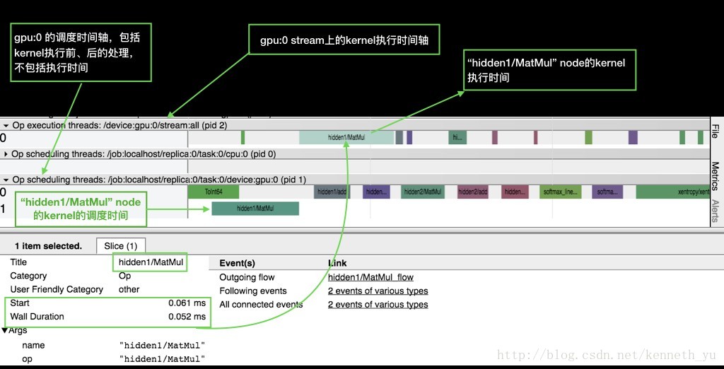
可以看到:
横向是时间轴:各device对graph node的kernel调度时间轴、执行时间轴。
整个graph中所有执行到的node在devices上的运行分布。由于本例中node缺省使用gpu:0,所以cpu:0上没有执行node的分布。
一个kernel的执行包括调度和执行两个阶段,这两个阶段是异步操作,所以我们看到同一个时间点, 当 gpu:0/stream 上还在执行hidden1/Matmul, 而gpu:0已经开始调度下一个node: hidden1/add 的kernel, 这样实现了最大程度上不同node 间的并发。
你可以通过tf.device()将部分node分布到其他gpu上或者cpu上,看看做model parallel的结果。
例子2:scope view显示模型中的参数数量分布
通过这种方式,查看各个layer中参数的总数,以控制模型的大小和参数分布。
我们得到param数量从高到低的排序显示:
最多的是:
hidden1/weights (784x128, 100.35k/100.35k params): 因为mnist数据集image的size是28*28=784, 我们定义的hidden1 layer的dim是128,所以w的大小 784*128 = 100,350.
hidden1/biases (128, 128/128 params):bias对应hidden1 layer的dim128.
例子3: op view显示模型中的expensive node
在一个graph中不同的node可能会用到相同的op,我们可以将这些node按照op进行归类、汇总,
检测op的执行时间、占用内存, 找到最耗时、或者最占内存的op,通过调整kernel算法、更换执行设备device的分布来优化。
比如,我们可以找出最耗时top 5 ops:
输出结果: 可以看到MatMul是最耗时的op, 占用了整个graph node总执行时间的40.98%.
op的exection time,是所有使用该op的node的execution time的总和。这里显示的时间是所有Run step的均值,其中:
accelerator execution time - 在gpu上的执行时间
cpu execution time - 调度时间
op occurrence - 使用该op的node个数
也可以找出最占用内存的top 5 ops:
输出结果:可以看到MatMul由于需要申请大量的buffer来保存中间结果和输出结果, 占用了整个graph node总消耗内存的99.62%.
例子4: code view – 显示python代码的执行资源消耗
按照python代码的方式来显示统计数据,也就是统计每一行python代码产生的node的执行性能。
显示结果:mnist.py:127行占用的执行时间最长,
这是因为我们在创建train_op时,tensorflow会自动创建Back Propagation的所有node,所以对应的执行时间也是最多的。
显示结果如下:
使用tensorflow profiler举例
高级功能Advisor
tensorflow profiler 主要特性
从r1.3版本开始, tensorflow 提供profiler模块,参见github上的官网文档为方便描述,下面将tf中运行的神经网络模型简称为graph,其中的节点称为node.
profiler的最大好处是:打开tf执行的黑盒,以graph node为最细的粒度,从多个维度、多个层面去统计神经网络运行的时间
和内存消耗,为进一步优化神经网络模型的运行效率提供最直接的数据依据。
profiler 分为数据搜集和数据显示两个主要步骤。
数据搜集
Created with Raphaël 2.1.0sessionsessionprofilerprofilerRun记录单步统计数据RunMetadata记录和处理
graph node的每一次执行,记录单步统计数据,主要是执行时间和占用内存,格式参见step_stats.proto,作为原始的最小粒度统计数据源;
每一次session.Run(),所有执行到的graph node的统计数据,都集中汇总保存到 RunMetadata 数据结构中;
用户程序把每一次搜集到的 RunMetadata 添加到profiler实例,做数据累计和加工处理。
数据显示: 数据的过滤、视图组织和显示输出
部分规则需要用户自己指定:
- 数据的过滤: 比如graph node过滤条件、 显示的字段、排序方式等。
四种视图: 对应显示节点之前的不同组织方式,下面我会结合例子描述。
graph view
scope view
op view
code view
视图输出方式:
time line : 输出JSON events file, 再用chrome浏览器tracing功能进行查看,可视性很棒。
stdout : 标准输出设备打印。
pprof file: 输出pprof的文件格式,再用pprof工具查看。
file: 输出到普通的文本文件。
视图和输出方式,可以自由组合,除了部分特例不能输出,比如op view 不支持time line输出,只有code view能够输出pprof格式的文件等,
详细规则参见 Options
使用tensorflow profiler举例
目前tf profiler的使用通过两种接口:python API
命令行
两者在提供的功能上面没有差别。
命令行方式需要编译一个profiler可执行文件,然后在shell运行这个可执行文件,进入其交互式界面,通过命令行操作。
这里以python API 为例讲解。
首先,确认下载安装了 r1.3 的python包。
网络模型使用简单的mnist.py .
为了调试方便,我们进入python3 console运行。
$ python3
Python 3.4.5 |Continuum Analytics, Inc.| (default, Jul  2 2016, 17:47:47)
[GCC 4.4.7 20120313 (Red Hat 4.4.7-1)] on linux
Type "help", "copyright", "credits" or "license" for more information.
>>>
下面的代码可以直接拷贝进python console运行。
import相关的包
import tensorflow as tf
from tensorflow.examples.tutorials.mnist import mnist
from tensorflow.examples.tutorials.mnist import input_data
from tensorflow.python.profiler import model_analyzer
from tensorflow.python.profiler import option_builder
定义模型相关参数
class FLAGS:
def __init__(self):
self.hidden1_dim =128     #hidden1 layer 的维度
self.hidden2_dim = 32     #hidden2 layer 的维度
self.learning_rate = 1e-2
self.batch_size = 100
self.max_step = 100        # 最大的训练步骤
self.stats_per_steps = 10  # 每隔10步搜集一次RunMetadata。 可以根据需要修改
self.data_set_dir =  '' #替换为你的本地mnist数据集路径,如果你已经下载过

TRAINING_FLAGS = FLAGS()
定义网络模型,创建session. 这段代码与tfprofiler无关,直接粘贴即可,不用读
网络模型不做修改,沿用原来的: hidden1 + hidden2 + softmax 三层架构, hidden1和hidden2都是(Wx+b)->Relu的路径。
在我的环境中默认都运行在gpu:0 上。
data_sets = input_data.read_data_sets(train_dir=TRAINING_FLAGS.data_set_dir,fake_data=False)
images_placeholder = tf.placeholder(tf.float32, shape=(TRAINING_FLAGS.batch_size,
mnist.IMAGE_PIXELS))
labels_placeholder = tf.placeholder(tf.int32, shape=(TRAINING_FLAGS.batch_size))

logits = mnist.inference(images_placeholder,
TRAINING_FLAGS.hidden1_dim,
TRAINING_FLAGS.hidden2_dim)
loss = mnist.loss(logits, labels_placeholder)
train_op = mnist.training(loss, TRAINING_FLAGS.learning_rate)
init = tf.global_variables_initializer()
sess = tf.Session()
sess.run(init)
创建tfprofiler实例,作为记录、处理和显示数据的主体
mnist_profiler = model_analyzer.Profiler(graph=sess.graph)
定义trace level为FULL_TRACE,这样我们才能搜集到包括GPU硬件在内的最全统计数据
run_options = tf.RunOptions(trace_level = tf.RunOptions.FULL_TRACE)
创建RunMetadata, 用于在每次session.Run()时汇总统计数据
run_metadata = tf.RunMetadata()
循环执行session.Run(),搜集统计数据并添加到tfprofiler实例中
feed_dict = dict()
for step in range(TRAINING_FLAGS.max_step):
images_feed, labels_feed = data_sets.train.next_batch(TRAINING_FLAGS.batch_size, fake_data=False)
feed_dict = {
images_placeholder: images_feed,
labels_placeholder: labels_feed,
}
#每 TRAINING_FLAGS.stats_per_steps 步,搜集一下统计数据:
if step % TRAINING_FLAGS.stats_per_steps == 0:
_, loss_value = sess.run(fetches=[train_op, loss],feed_dict=feed_dict, options=run_options, run_metadata=run_metadata)

#将本步搜集的统计数据添加到tfprofiler实例中
mnist_profiler.add_step(step=step, run_meta=run_metadata)
else:
_, loss_value = sess.run(fetches=[train_op, loss],
feed_dict=feed_dict)
接下来我们就可以显示统计视图了
定义显示option 和 视图方式
option用于设置过滤条件、显示字段,完整option 参见Options,常用设置项目:
account_type_regexes:采用Google RE2规则的正则表达式,
过滤要显示的node的op type 和 device,比如 ‘.MatMul.‘, ‘.*Conv2D’, ‘.*gpu:0’等。
select:要显示的字段:
[bytes|micros|accelerator_micros|cpu_micros|params|float_ops|occurrence|tensor_value|device|op_types|input_shapes]
order_by: 显示结果排序方式:
[name|depth|bytes|micros|accelerator_micros|cpu_micros|params|float_ops|occurrence]
output: 输出方式:stdout, file 或者 timeline。
step: 显示在某个具体的Run() step的统计值. 缺省值-1,显示所有步骤的平均值。
一般来说, option和试图总是结合起来使用,这里举几个典型应用例子:
例子1:grpah view显示每个graph node运行时间,并输出到timeline
#统计内容为每个graph node的运行时间和占用内存
profile_graph_opts_builder = option_builder.ProfileOptionBuilder(
option_builder.ProfileOptionBuilder.time_and_memory())

#输出方式为timeline
profile_graph_opts_builder.with_timeline_output(timeline_file='/tmp/mnist_profiler.json')
#定义显示sess.Run() 第70步的统计数据
profile_graph_opts_builder.with_step(70)

#显示视图为graph view
mnist_profiler.profile_graph(profile_graph_opts_builder.build())
我们得到第70步的详细time line结果,打开chrome浏览器,输入about:tracing, 然后load “/tmp/mnist_profiler.json” 文件,这时候可以看见time line的显示结果。
chrome tracing简介参考这篇文章:In-depth: Using Chrome://tracing to view your inline profiling data
截屏如下:
可以看到:
横向是时间轴:各device对graph node的kernel调度时间轴、执行时间轴。
整个graph中所有执行到的node在devices上的运行分布。由于本例中node缺省使用gpu:0,所以cpu:0上没有执行node的分布。
一个kernel的执行包括调度和执行两个阶段,这两个阶段是异步操作,所以我们看到同一个时间点, 当 gpu:0/stream 上还在执行hidden1/Matmul, 而gpu:0已经开始调度下一个node: hidden1/add 的kernel, 这样实现了最大程度上不同node 间的并发。
你可以通过tf.device()将部分node分布到其他gpu上或者cpu上,看看做model parallel的结果。
例子2:scope view显示模型中的参数数量分布
通过这种方式,查看各个layer中参数的总数,以控制模型的大小和参数分布。
#统计内容为所有trainable Variable Op
profile_scope_opt_builder = option_builder.ProfileOptionBuilder(
option_builder.ProfileOptionBuilder.trainable_variables_parameter())

#显示的嵌套深度为4
profile_scope_opt_builder.with_max_depth(4)
#显示字段是params,即参数
profile_scope_opt_builder.select(['params'])
#根据params数量进行显示结果排序
profile_scope_opt_builder.order_by('params')

#显示视图为scope view
mnist_profiler.profile_name_scope(profile_scope_opt_builder.build())
我们得到param数量从高到低的排序显示:
==================Model Analysis Report======================
node name | # parameters
_TFProfRoot (--/104.94k params)
hidden1 (--/100.48k params)
hidden1/weights (784x128, 100.35k/100.35k params)
hidden1/biases (128, 128/128 params)
hidden2 (--/4.13k params)
hidden2/weights (128x32, 4.10k/4.10k params)
hidden2/biases (32, 32/32 params)
softmax_linear (--/330 params)
softmax_linear/weights (32x10, 320/320 pa
da3d
rams)
softmax_linear/biases (10, 10/10 params)

======================End of Report==========================
最多的是:
hidden1/weights (784x128, 100.35k/100.35k params): 因为mnist数据集image的size是28*28=784, 我们定义的hidden1 layer的dim是128,所以w的大小 784*128 = 100,350.
hidden1/biases (128, 128/128 params):bias对应hidden1 layer的dim128.
例子3: op view显示模型中的expensive node
在一个graph中不同的node可能会用到相同的op,我们可以将这些node按照op进行归类、汇总,
检测op的执行时间、占用内存, 找到最耗时、或者最占内存的op,通过调整kernel算法、更换执行设备device的分布来优化。
比如,我们可以找出最耗时top 5 ops:
profile_op_opt_builder = option_builder.ProfileOptionBuilder()

#显示字段:op执行时间,使用该op的node的数量。 注意:op的执行时间即所有使用该op的node的执行时间总和。
profile_op_opt_builder.select(['micros','occurrence'])
#根据op执行时间进行显示结果排序
profile_op_opt_builder.order_by('micros')
#过滤条件:只显示排名top 5
profile_op_opt_builder.with_max_depth(4)

#显示视图为op view
mnist_profiler.profile_operations(profile_op_opt_builder.build())
输出结果: 可以看到MatMul是最耗时的op, 占用了整个graph node总执行时间的40.98%.
op的exection time,是所有使用该op的node的execution time的总和。这里显示的时间是所有Run step的均值,其中:
accelerator execution time - 在gpu上的执行时间
cpu execution time - 调度时间
op occurrence - 使用该op的node个数
==================Model Analysis Report======================
node name | total execution time | accelerator execution time | cpu execution time | op occurrence (run|defined)
MatMul                          509us (100.00%, 40.98%),        169us (100.00%, 65.76%),        336us (100.00%, 34.53%),        9|9
ApplyGradientDescent             151us (59.02%, 12.16%),           17us (34.24%, 6.61%),         132us (65.47%, 13.57%),        6|6
Sum                               111us (46.86%, 8.94%),           12us (27.63%, 4.67%),          99us (51.90%, 10.17%),        6|6
SparseSoftmaxCrossEntropyWithLogits         110us (37.92%, 8.86%),          26us (22.96%, 10.12%),           83us (41.73%, 8.53%),        1|1
Add                                78us (29.07%, 6.28%),           11us (12.84%, 4.28%),           66us (33.20%, 6.78%),        3|6

======================End of Report==========================
也可以找出最占用内存的top 5 ops:
profile_op_opt_builder = option_builder.ProfileOptionBuilder()

#显示字段:op占用内存,使用该op的node的数量。 注意:op的占用内存即所有使用该op的node的占用内存总和。
profile_op_opt_builder.select(['bytes','occurrence'])
#根据op占用内存进行显示结果排序
profile_op_opt_builder.order_by('bytes')
#过滤条件:只显示排名最靠前的5个op
profile_op_opt_builder.with_max_depth(4)

#显示视图为op view
mnist_profiler.profile_operations(profile_op_opt_builder.build())
输出结果:可以看到MatMul由于需要申请大量的buffer来保存中间结果和输出结果, 占用了整个graph node总消耗内存的99.62%.
==================Model Analysis Report======================
node name | requested bytes | op occurrence (run|defined)
MatMul                       866.05KB (100.00%, 99.62%),        9|9
Sum                               1.02KB (0.38%, 0.12%),        6|6
Cast                              1.02KB (0.27%, 0.12%),        1|2
SparseSoftmaxCrossEntropyWithLogits         1.02KB (0.15%, 0.12%),        1|1
Mean                                256B (0.03%, 0.03%),        1|1

======================End of Report==========================
例子4: code view – 显示python代码的执行资源消耗
按照python代码的方式来显示统计数据,也就是统计每一行python代码产生的node的执行性能。
profile_code_opt_builder = option_builder.ProfileOptionBuilder()

#过滤条件:显示minist.py代码。
profile_code_opt_builder.with_max_depth(1000)
profile_code_opt_builder.with_node_names(show_name_regexes=['mnist.py.*'])

#过滤条件:只显示执行时间大于10us的代码
profile_code_opt_builder.with_min_execution_time(min_micros=10)

#显示字段:执行时间,且结果按照时间排序
profile_code_opt_builder.select(['micros'])
profile_code_opt_builder.order_by('micros')

#显示视图为code view
mnist_profiler.profile_python(profile_code_opt_builder.build())
显示结果:mnist.py:127行占用的执行时间最长,
这是因为我们在创建train_op时,tensorflow会自动创建Back Propagation的所有node,所以对应的执行时间也是最多的。
==================Model Analysis Report======================
node name | total execution time | accelerator execution time | cpu execution time
_TFProfRoot (--/1.44ms, --/249us, --/1.18ms)
mnist.py:127:training:train_op = optimi... (0us/790us, 0us/133us, 0us/652us)
mnist.py:64:inference:hidden1 = tf.nn.r... (0us/209us, 0us/57us, 0us/152us)
mnist.py:98:loss:labels=labels, lo... (0us/132us, 0us/23us, 0us/108us)
mnist.py:73:inference:hidden2 = tf.nn.r... (0us/109us, 0us/24us, 0us/83us)
mnist.py:82:inference:logits = tf.matmu... (0us/66us, 0us/7us, 0us/59us)
mnist.py:96:loss:labels = tf.to_in... (0us/47us, 0us/2us, 0us/45us)
mnist.py:99:loss:return tf.reduce_... (0us/38us, 0us/3us, 0us/35us)
mnist.py:124:training:global_step = tf.... (0us/10us, 0us/0us, 0us/10us)

======================End of Report==========================
高级功能Advisor
tf.profiler 实例自动输出检测结果,给出优化建议。mnist_profiler.advise(options=model_analyzer.ALL_ADVICE)
显示结果如下:
ExpensiveOperationChecker:
top 1 operation type: MatMul, cpu: 352us, accelerator: 167us, total: 521us (38.85%)
top 2 operation type: ApplyGradientDescent, cpu: 140us, accelerator: 16us, total: 159us (11.86%)
top 3 operation type: Sum, cpu: 110us, accelerator: 12us, total: 123us (9.17%)
top 1 graph node: gradients, cpu: 0us, accelerator: 0us, total: 0us
top 2 graph node: hidden1, cpu: 0us, accelerator: 0us, total: 0us
top 3 graph node: GradientDescent, cpu: 4us, accelerator: 0us, total: 4us

OperationChecker:

AcceleratorUtilizationChecker:
device: /job:localhost/replica:0/task:0/device:gpu:0 low utilization: 0.17

相关文章推荐
- 使用循环神经网络实现语言模型——源自《TensorFlow:实战Goole深度学习框架》
- 使用Tensorflow训练神经网络模型---自定义损失函数
- 使用TensorFlow训练循环神经网络语言模型
- Tensorflow 核心流程剖析 3-- 运行设备Device的生成和管理
- 使用 libevent 和 libev 提高网络应用性能——I/O模型演进变
- 使用Matlab结合神经网络模型对多波段影像进行计算
- 基于回归神经网络的中文语句模型实践(Python+Tensorflow+阿里云)
- 使用 libevent 和 libev 提高网络应用性能——I/O模型演进变化史
- 网络采集软件核心技术剖析系列(3)---如何使用C#语言下载博文中的全部图片到本地并可以离线浏览
- 【神经网络与深度学习】Caffe使用step by step:使用自己数据对已经训练好的模型进行finetuning
- Tensorflow搭建神经网络及使用Tensorboard进行可视化
- 基于回归神经网络的中文语句模型实践(Python+Tensorflow+阿里云)
- 机器学习的大局观:使用神经网络和TensorFlow来对文本分类
- 使用 全连接神经网络 和 词袋模型 进行文本分类的example
- 使用python写神经网络模型之分类器
- 网络采集软件核心技术剖析系列(1)---如何使用C#语言获取博客园某个博主的全部随笔链接及标题
- 使用 libevent 和 libev 提高网络应用性能——I/O模型演进变化史
- ANN_MLP神经网络使用流程详述
- 网络采集软件核心技术剖析系列(7)---如何使用C#语言搭建程序框架(经典Winform界面,顶部菜单栏,工具栏,左边树形列表,右边多Tab界面)
- mininet安装与使用,wireshark抓包器, iperf网络性能检测