使用腾讯云 GPU 学习深度学习系列之四：深度学习的特征工程

这是《使用腾讯云GPU学习深度学习》系列文章的第四篇，主要举例介绍了深度学习计算过程中的一些数据预处理方法。本系列文章主要介绍如何使用 腾讯云GPU服务器 进行深度学习运算，前面主要介绍原理部分，后期则以实践为主。

往期内容：
使用腾讯云 GPU 学习深度学习系列之一：传统机器学习的回顾

使用腾讯云 GPU 学习深度学习系列之二：Tensorflow 简明原理

使用腾讯云 GPU 学习深度学习系列之三：搭建深度神经网络

上一节，我们基于

Keras

设计了一个用于 CIFAR-10 数据集的深度学习网络。我们的代码主要包括以下部分：
批量输入模块
各种深度学习零件搭建的深度神经网络
凸优化模块
模型的训练与评估

我们注意到，批量输入模块中，实际上就是运用了一个生成器，用来批量读取图片文件，保存成矩阵，直接用于深度神经网络的训练。由于在训练的过程中，图片的特征，是由卷积神经网络自动获取的，因此深度学习通常被认为是一种 端对端（End
to end） 的训练方式，期间不需要人为的过多干预。

但是，在实际的运用过程中，这一条并不总是成立。深度神经网络在某些特定的情况下，是需要使用某些特定方法，在批量输入模块之前，对输入数据进行预处理，并且处理结果会极大的改善。

本讲将主要介绍几种数据预处理方法，并且通过这些预处理方法，进行特征提取，提升模型的准确性。

1. 结合传统数据处理方法的特征提取

这一部分我们举医学影像学的一个例子，以 Kaggle 社区第三届数据科学杯比赛的肺部 CT 扫描结节数据为例，来说明如何进行数据的前处理。以下代码改编自该
kaggle 比赛的官方指导教程,主要是特异性的提取 CT 影像图片在肺部的区域的扫描结果，屏蔽无关区域，进而对屏蔽其他区域后的结果，使用深度学习方法进行进一步分析。

屏蔽的程序本身其实并未用到深度学习相关内容，这里主要使用了

skimage

库。下面我们详细介绍一下具体方法。

第一步，读取医学影像图像。这里以 LUNA16数据集 中的

1.3.6.1.4.1.14519.5.2.1.6279.6001.179049373636438705059720603192

 这张CT
影像数据为例，这张片子可以在这里下载，然后解压缩，用下面的代码分析。其他片子请在 LUNA16
数据集)下载：

from __future__ import print_function, division

import numpy as np
import os
import csv
from glob import glob
import pandas as pd
import numpy as np
import SimpleITK as sitk

from skimage import measure,morphology
from sklearn.cluster import KMeans
from skimage.transform import resize
import matplotlib.pyplot as plt
import seaborn as sns

from glob import glob

try:
from tqdm import tqdm # long waits are not fun
except:
print('TQDM does make much nicer wait bars...')
tqdm = lambda x: x

def make_mask(center,diam,z,width,height,spacing,origin):
'''
Center : centers of circles px -- list of coordinates x,y,z
diam : diameters of circles px -- diameter
widthXheight : pixel dim of image
spacing = mm/px conversion rate np array x,y,z
origin = x,y,z mm np.array
z = z position of slice in world coordinates mm
'''
mask = np.zeros([height,width]) # 0's everywhere except nodule swapping x,y to match img
#convert to nodule space from world coordinates

# Defining the voxel range in which the nodule falls
v_center = (center-origin)/spacing
v_diam = int(diam/spacing[0]+5)
v_xmin = np.max([0,int(v_center[0]-v_diam)-5])
v_xmax = np.min([width-1,int(v_center[0]+v_diam)+5])
v_ymin = np.max([0,int(v_center[1]-v_diam)-5])
v_ymax = np.min([height-1,int(v_center[1]+v_diam)+5])

v_xrange = range(v_xmin,v_xmax+1)
v_yrange = range(v_ymin,v_ymax+1)

# Convert back to world coordinates for distance calculation
x_data = [x*spacing[0]+origin[0] for x in range(width)]
y_data = [x*spacing[1]+origin[1] for x in range(height)]

# Fill in 1 within sphere around nodule
for v_x in v_xrange:
for v_y in v_yrange:
p_x = spacing[0]*v_x + origin[0]
p_y = spacing[1]*v_y + origin[1]
if np.linalg.norm(center-np.array([p_x,p_y,z]))<=diam:
mask[int((p_y-origin[1])/spacing[1]),int((p_x-origin[0])/spacing[0])] = 1.0
return(mask)

def matrix2int16(matrix):
'''
matrix must be a numpy array NXN
Returns uint16 version
'''
m_min= np.min(matrix)
m_max= np.max(matrix)
matrix = matrix-m_min
return(np.array(np.rint( (matrix-m_min)/float(m_max-m_min) * 65535.0),dtype=np.uint16))

df_node = pd.read_csv('./annotation.csv')
for fcount, img_file in enumerate(tqdm(df_node['seriesuid'])):
mini_df = df_node[df_node["seriesuid"]==img_file] #get all nodules associate with file
if mini_df.shape[0]>0: # some files may not have a nodule--skipping those
# load the data once
itk_img = sitk.ReadImage("%s.mhd" % img_file)
img_array = sitk.GetArrayFromImage(itk_img) # indexes are z,y,x (notice the ordering)
num_z, height, width = img_array.shape        #heightXwidth constitute the transverse plane
origin = np.array(itk_img.GetOrigin())      # x,y,z  Origin in world coordinates (mm)
spacing = np.array(itk_img.GetSpacing())    # spacing of voxels in world coor. (mm)
# go through all nodes (why just the biggest?)
for node_idx, cur_row in mini_df.iterrows():
node_x = cur_row["coordX"]
node_y = cur_row["coordY"]
node_z = cur_row["coordZ"]
diam = cur_row["diameter_mm"]
# just keep 3 slices
imgs = np.ndarray([3,height,width],dtype=np.float32)
masks = np.ndarray([3,height,width],dtype=np.uint8)
center = np.array([node_x, node_y, node_z])   # nodule center
v_center = np.rint((center-origin)/spacing)  # nodule center in voxel space (still x,y,z ordering)
for i, i_z in enumerate(np.arange(int(v_center[2])-1,
int(v_center[2])+2).clip(0, num_z-1)): # clip prevents going out of bounds in Z
mask = make_mask(center, diam, i_z*spacing[2]+origin[2],
width, height, spacing, origin)
masks[i] = mask
imgs[i] = img_array[i_z]
np.save(os.path.join("./images_%04d_%04d.npy" % (fcount,node_idx)),imgs)
np.save(os.path.join("./masks_%04d_%04d.npy"  % (fcount,node_idx)),masks)

简单解释下，首先，CT 影像是一个三维的图像，以三维矩阵的形式保存在

1.3.6.1.4.1.14519.5.2.1.6279.6001.179049373636438705059720603192.raw

 这个文件中，

.mhd

文件则保存了影像文件的基本信息。具体而言，

annotation.csv

 文件中，图像中结节的坐标是：

x	seriesuid	coordX	coordY	coordZ	diameter_mm
0	1.3.6.1.4.1.14519.5.2.1.6279.6001.179049373636...	56.208405	86.343413	-115.867579	23.350644

这里结节坐标的 coordX~Z 都是物理坐标， 

.mhd

文件保存的，就是从这些物理坐标到 

.raw

文件中矩阵坐标的映射。于是上面整个函数，其实就是在从
CT 影像仪器的原始文件读取信息，转换物理坐标为矩阵坐标，并且 将结节附近的CT 切片存储成对应的 python 矩阵，用来进行进一步的分析。

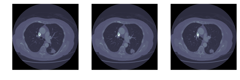
然后，我们看一下读取的结果。可见输入文件中标注的结节就在右下方。

img_file = "./images_0000_0000.npy"
imgs_to_process = np.load(img_file).astype(np.float64)

fig = plt.figure(figsize=(12,4))
for i in range(3):
ax = fig.add_subplot(1,3,i+1)
ax.imshow(imgs_to_process[i,:,:], 'bone')
ax.set_axis_off()

可见图中，除了中间亮度较低的肺部，还有亮度较高的脊柱、肋骨，以及肌肉、脂肪等组织。我们的一个思路，就是 留下暗的区域，去掉亮的区域。当然这里，亮度多高才算亮？这个我们可以对一张图中所有像素点的亮度做概率密度分布，然后用 

Kmeans

 算法，找出这个明暗分解的阈值(下文图中左上角)：

i = 0
img = imgs_to_process[i]

#Standardize the pixel values
mean = np.mean(img)
std = np.std(img)
img = img-mean
img = img/std

# Find the average pixel value near the lungs
#         to renormalize washed out images
middle = img[100:400,100:400]
mean = np.mean(middle)
max = np.max(img)
min = np.min(img)

# To improve threshold finding, I'm moving the
#         underflow and overflow on the pixel spectrum
img[img==max]=mean
img[img==min]=mean

# Using Kmeans to separate foreground (radio-opaque tissue)
#     and background (radio transparent tissue ie lungs)
# Doing this only on the center of the image to avoid
#     the non-tissue parts of the image as much as possible
kmeans = KMeans(n_clusters=2).fit(np.reshape(middle,[np.prod(middle.shape),1]))
centers = sorted(kmeans.cluster_centers_.flatten())
threshold = np.mean(centers)
thresh_img = np.where(img<threshold,1.0,0.0)  # threshold the image

然后使用 

skimage

 工具包。 skimage 是python一种传统图像处理的工具，我们这里，主要使用这个工具包，增强图像的轮廓，去除图像的细节，进而根据图像的轮廓信息，进行图像的分割，得到目标区域（Region
of Interests, ROI）。

# 对一张图中所有像素点的亮度做概率密度分布, 用竖线标注阈值所在
fig = plt.figure(figsize=(8,12))
ax1 = fig.add_subplot(321)
sns.distplot(middle.ravel(), ax=ax1)
ax1.vlines(x=threshold, ymax=10, ymin=0)
ax1.set_title('Threshold: %1.2F' % threshold)
ax1.set_xticklabels([])

# 展示阈值对图像切割的结果。小于阈值的点标注为1，白色。大于阈值的点标注为0，黑色。
ax2 = fig.add_subplot(322)
ax2.imshow(thresh_img, "gray")
ax2.set_axis_off()
ax2.set_title('Step1, using threshold as cutoff')

# 增大黑色部分（非ROI）的区域，使之尽可能的连在一起
eroded = morphology.erosion(thresh_img,np.ones([4,4]))
ax3 = fig.add_subplot(323)
ax3.imshow(eroded, "gray")
ax3.set_axis_off()
ax3.set_title('Step2,  erosion shrinks bright\nregions and enlarges dark regions.')

# 增大白色部分（ROI）的区域，尽可能的消除面积较小的黑色区域
dilation = morphology.dilation(eroded,np.ones([10,10]))
ax4 = fig.add_subplot(324)
ax4.imshow(dilation, "gray")
ax4.set_axis_off()
ax4.set_title('Step3,  dilation shrinks dark\nregions and enlarges bright regions.')

# 上一张图中共有三片连续区域，即最外层的体外区域，内部的肺部区域，以及二者之间的身体轮廓区域。这里将其分别标出
labels = measure.label(dilation)
ax5 = fig.add_subplot(325)
ax5.imshow(labels, "gray")
#ax5.set_axis_off()
ax5.set_title('Step4, label connected regions\n of an integer array.')

# 提取regions 信息，这张图片的 region的 bbox位置分别在 [[0,0,512,512],[141, 86, 396, 404]],
#   分别对应 体外+轮廓 以及 肺部区域的左上角、右下角坐标。
#   于是这里通过区域的宽度 B[2]-B[0]、高度 B[3]-B[1]
#   以及距离图片上下的距离  B[0]>40 and B[2]<472,
#   最终保留需要的区域。
regions = measure.regionprops(labels)
good_labels = []
for prop in regions:
B = prop.bbox
if B[2]-B[0]<475 and B[3]-B[1]<475 and B[0]>40 and B[2]<472:
good_labels.append(prop.label)

mask = np.zeros_like(labels)
for N in good_labels:
mask = mask + np.where(labels==N,1,0)

mask = morphology.dilation(mask,np.ones([10,10])) # one last dilation

ax6 = fig.add_subplot(326)
ax6.imshow(mask, "gray")
ax6.set_axis_off()
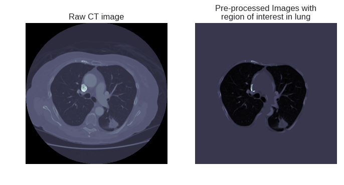
ax6.set_title('Step5, remain the region of interests.')

最后再看一下提取的效果如何：

fig = plt.figure(figsize=(8,4))

ax1 = fig.add_subplot(1,2,1)
ax1.imshow(imgs_to_process[0,:,:], 'bone')
ax1.set_axis_off()
ax1.set_title("Raw CT image")

ax2 = fig.add_subplot(1,2,2)
ax2.imshow(imgs_to_process[0,:,:]*mask, 'bone')
ax2.set_axis_off()
ax2.set_title("Pre-processed Images with\nregion of interest in lung")

右图将进一步的放入深度学习模型，进行肺部结节的进一步检测。

2. 结合深度学习技术的特征提取增强

除了通过传统手段进行数据预先处理，我们同样可以使用深度学习技术进行这一步骤。

可能大家对手写数字识别数据集（MNIST）非常熟悉，Tensorflow 官网就有教程，指导如何搭建卷积神经网络，训练一个准确率高达
99.2% 的模型。



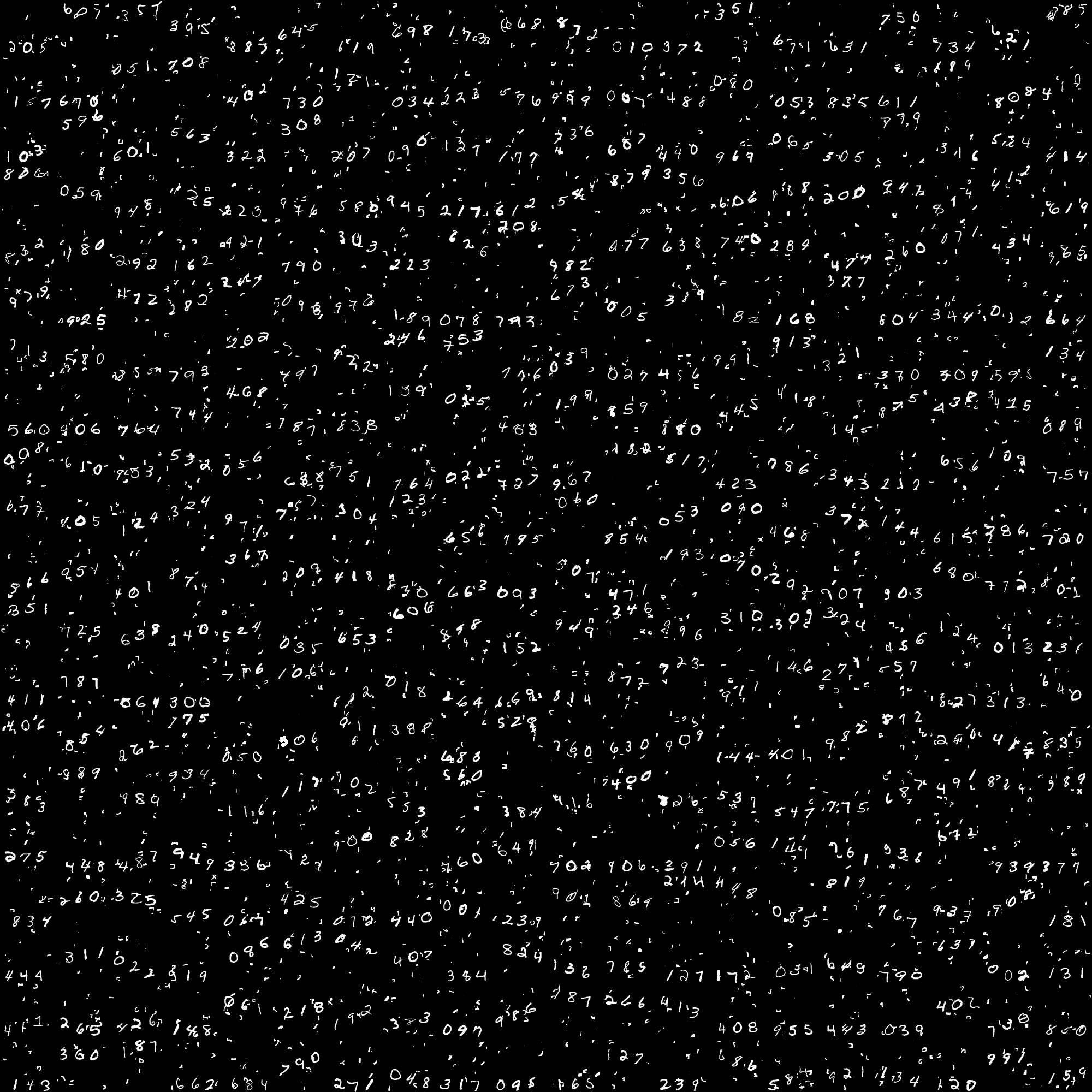
但实际运用过程中，我们会发现其实 MNIST 数据集其实书写的比较工整，于是我们就考虑到，对于比较潦草的书写，直接训练卷积神经网络，是否是最好的选择？是否可以将“草书”字体的数字，变得正规一点，然后放进卷积神经网络训练？于是我们利用一个“草书”版的 MNIST 数据集，来介绍一下

spatial_transform

 模块：

首先需要下载这个“草书”版的手写数字集：

wget https://github.com/daviddao/spatial-transformer-tensorflow/raw/master/data/mnist_sequence1_sample_5distortions5x5.npz

画风如下，明显凌乱了许多，但其实人还是可以看懂，所以我们可以尝试使用深度神经网络来解决。



我们开始分析数据。首先读数据：

import tensorflow as tf
# https://github.com/tensorflow/models/tree/master/transformer from spatial_transformer import transformer
import numpy as np
from tf_utils import weight_variable, bias_variable, dense_to_one_hot
import matplotlib.pyplot as plt
from keras.backend.tensorflow_backend import set_session

np.random.seed(0)
tf.set_random_seed(0)

config = tf.ConfigProto()
config.gpu_options.allow_growth=True
set_session(tf.Session(config=config))
%matplotlib inline

mnist_cluttered = np.load('./mnist_sequence1_sample_5distortions5x5.npz')

X_train = mnist_cluttered['X_train']
y_train = mnist_cluttered['y_train']
X_valid = mnist_cluttered['X_valid']
y_valid = mnist_cluttered['y_valid']
X_test = mnist_cluttered['X_test']
y_test = mnist_cluttered['y_test']

Y_train = dense_to_one_hot(y_train, n_classes=10)
Y_valid = dense_to_one_hot(y_valid, n_classes=10)
Y_test = dense_to_one_hot(y_test, n_classes=10)

初始化参数，然后直接得到一批原始数据，放入

xout

：

x = tf.placeholder(tf.float32, [None, 1600])
keep_prob = tf.placeholder(tf.float32)

iter_per_epoch = 100
n_epochs = 500
train_size = 10000
indices = np.linspace(0, 10000 - 1, iter_per_epoch)
indices = indices.astype('int')
iter_i = 0

batch_xs = X_train[indices[iter_i]:indices[iter_i+1]]
x_tensor = tf.reshape(x, [-1, 40, 40, 1])

sess = tf.Session()
sess.run(tf.global_variables_initializer())
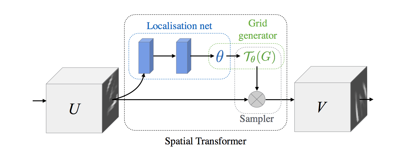
xout = sess.run(x_tensor, feed_dict={x: batch_xs})

然后搭建一个 

spatial_transform

 网络。网络结构如下图：

x = tf.placeholder(tf.float32, [None, 1600])
y = tf.placeholder(tf.float32, [None, 10])

x_tensor = tf.reshape(x, [-1, 40, 40, 1])
W_fc_loc1 = weight_variable([1600, 20])
b_fc_loc1 = bias_variable([20])

W_fc_loc2 = weight_variable([20, 6])
initial = np.array([[1., 0, 0], [0, 1., 0]])
initial = initial.astype('float32')
initial = initial.flatten()
b_fc_loc2 = tf.Variable(initial_value=initial, name='b_fc_loc2')

# %% Define the two layer localisation network
h_fc_loc1 = tf.nn.tanh(tf.matmul(x, W_fc_loc1) + b_fc_loc1)

# %% We can add dropout for regularizing and to reduce overfitting like so:
keep_prob = tf.placeholder(tf.float32)
h_fc_loc1_drop = tf.nn.dropout(h_fc_loc1, keep_prob)

# %% Second layer
h_fc_loc2 = tf.nn.tanh(tf.matmul(h_fc_loc1_drop, W_fc_loc2) + b_fc_loc2)

# %% We'll create a spatial transformer module to identify discriminative
# %% patches
out_size = (40, 40)
h_trans = transformer(x_tensor, h_fc_loc2, out_size)

再得到一批经过变换后的数据，放入

xtransOut

：

iter_i = 0
batch_xs = X_train[0:101]
batch_ys = Y_train[0:101]

sess = tf.Session()
sess.run(tf.global_variables_initializer())

xtransOut = sess.run(h_trans,
feed_dict={
x: batch_xs,
y: batch_ys,
keep_prob: 1.0
})

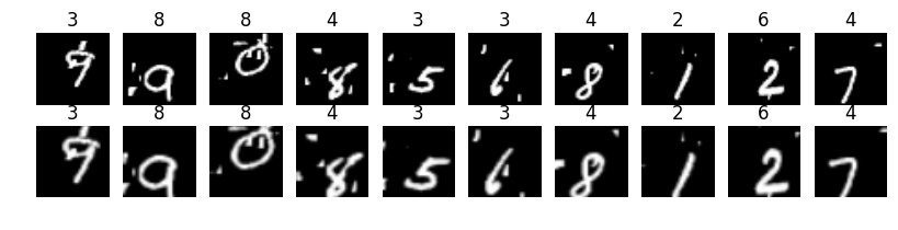
展示两批数据。上面一行是原始数据，下面一行是变换后的数据。可见数字在局部被放大，有的数字写的歪的被自动正了过来：

fig = plt.figure(figsize=(10,2))

for idx in range(10):
ax1 = fig.add_subplot(2,10,idx+1)
ax2 = fig.add_subplot(2,10,idx+11)

ax1.imshow(xout[idx,:,:,0], "gray")
ax2.imshow(xtransOut[idx,:,:,0], "gray")
ax1.set_axis_off()
ax2.set_axis_off()
ax1.set_title(np.argmax(batch_ys, axis=1)[idx])
ax2.set_title(np.argmax(batch_ys, axis=1)[idx])

也就是说，通过 

spatial_transform

 层，对同一批输入数据的参数学习，我们最后实际上得到了一个坐标的映射 

Grid
generator

$T_{\theta(G)}$ ，可以将一个倾斜的、“草书”书写的数字，变得更正一点。



接下来，我们构建一个卷积神经网络:

x = tf.placeholder(tf.float32, [None, 1600])
y = tf.placeholder(tf.float32, [None, 10])
keep_prob = tf.placeholder(tf.float32)

def Networks(x,keep_prob, SpatialTrans=True):
x_tensor = tf.reshape(x, [-1, 40, 40, 1])
W_fc_loc1 = weight_variable([1600, 20])
b_fc_loc1 = bias_variable([20])

W_fc_loc2 = weight_variable([20, 6])
initial = np.array([[1., 0, 0], [0, 1., 0]])
initial = initial.astype('float32')
initial = initial.flatten()
b_fc_loc2 = tf.Variable(initial_value=initial, name='b_fc_loc2')

# %% Define the two layer localisation network
h_fc_loc1 = tf.nn.tanh(tf.matmul(x, W_fc_loc1) + b_fc_loc1)
# %% We can add dropout for regularizing and to reduce overfitting like so:

h_fc_loc1_drop = tf.nn.dropout(h_fc_loc1, keep_prob)
# %% Second layer
h_fc_loc2 = tf.nn.tanh(tf.matmul(h_fc_loc1_drop, W_fc_loc2) + b_fc_loc2)

# %% We'll create a spatial transformer module to identify discriminative
# %% patches
out_size = (40, 40)
h_trans = transformer(x_tensor, h_fc_loc2, out_size)

# %% We'll setup the first convolutional layer
# Weight matrix is [height x width x input_channels x output_channels]
filter_size = 3
n_filters_1 = 16
W_conv1 = weight_variable([filter_size, filter_size, 1, n_filters_1])

# %% Bias is [output_channels]
b_conv1 = bias_variable([n_filters_1])

# %% Now we can build a graph which does the first layer of convolution:
# we define our stride as batch x height x width x channels
# instead of pooling, we use strides of 2 and more layers
# with smaller filters.
if SpatialTrans:
h_conv1 = tf.nn.relu(
tf.nn.conv2d(input=h_trans,
filter=W_conv1,
strides=[1, 2, 2, 1],
padding='SAME') +
b_conv1)
else:
h_conv1 = tf.nn.relu(
tf.nn.conv2d(input=x_tensor,
filter=W_conv1,
strides=[1, 2, 2, 1],
padding='SAME') +
b_conv1)

# %% And just like the first layer, add additional layers to create
# a deep net
n_filters_2 = 16
W_conv2 = weight_variable([filter_size, filter_size, n_filters_1, n_filters_2])
b_conv2 = bias_variable([n_filters_2])
h_conv2 = tf.nn.relu(
tf.nn.conv2d(input=h_conv1,
filter=W_conv2,
strides=[1, 2, 2, 1],
padding='SAME') +
b_conv2)

# %% We'll now reshape so we can connect to a fully-connected layer:
h_conv2_flat = tf.reshape(h_conv2, [-1, 10 * 10 * n_filters_2])

# %% Create a fully-connected layer:
n_fc = 1024
W_fc1 = weight_variable([10 * 10 * n_filters_2, n_fc])
b_fc1 = bias_variable([n_fc])
h_fc1 = tf.nn.relu(tf.matmul(h_conv2_flat, W_fc1) + b_fc1)

h_fc1_drop = tf.nn.dropout(h_fc1, keep_prob)

# %% And finally our softmax layer:
W_fc2 = weight_variable([n_fc, 10])
b_fc2 = bias_variable([10])
y_logits = tf.matmul(h_fc1_drop, W_fc2) + b_fc2
return y_logits

# %% We'll now train in minibatches and report accuracy, loss:
iter_per_epoch = 100
n_epochs = 100
train_size = 10000

indices = np.linspace(0, 10000 - 1, iter_per_epoch)
indices = indices.astype('int')

首先训练一个未经过变换的：

y_logits_F = Networks(x, keep_prob, SpatialTrans=False)
cross_entropy_F = tf.reduce_mean(tf.nn.softmax_cross_entropy_with_logits(logits=y_logits_F, labels=y))
opt = tf.train.AdamOptimizer()
optimizer_F = opt.minimize(cross_entropy_F)
grads_F = opt.compute_gradients(cross_entropy_F, [b_fc_loc2])
correct_prediction_F = tf.equal(tf.argmax(y_logits_F, 1), tf.argmax(y, 1))
accuracy_F = tf.reduce_mean(tf.cast(correct_prediction_F, 'float'))

sessF = tf.Session()
sessF.run(tf.global_variables_initializer())

l_acc_F = []
for epoch_i in range(n_epochs):
for iter_i in range(iter_per_epoch - 1):
batch_xs = X_train[indices[iter_i]:indices[iter_i+1]]
batch_ys = Y_train[indices[iter_i]:indices[iter_i+1]]
sessF.run(optimizer_F, feed_dict={
x: batch_xs, y: batch_ys, keep_prob: 0.8})

acc = sessF.run(accuracy_F,
feed_dict={
x: X_valid,
y: Y_valid,
keep_prob: 1.0
})
l_acc_F.append(acc)
if epoch_i % 10 == 0:
print('Accuracy (%d): ' % epoch_i + str(acc))

Accuracy (0): 0.151
Accuracy (10): 0.813
Accuracy (20): 0.832
Accuracy (30): 0.825
Accuracy (40): 0.833
Accuracy (50): 0.837
Accuracy (60): 0.832
Accuracy (70): 0.837
Accuracy (80): 0.833
Accuracy (90): 0.843

可见这个神经网络对直接输入变形数据效果不好。我们再训练一个进过变换的：

y_logits = Networks(x, keep_prob)
cross_entropy = tf.reduce_mean(tf.nn.softmax_cross_entropy_with_logits(logits=y_logits, labels=y))
opt = tf.train.AdamOptimizer()
optimizer = opt.minimize(cross_entropy)
grads = opt.compute_gradients(cross_entropy, [b_fc_loc2])
correct_prediction = tf.equal(tf.argmax(y_logits, 1), tf.argmax(y, 1))
accuracy = tf.reduce_mean(tf.cast(correct_prediction, 'float'))

sess = tf.Session()
sess.run(tf.global_variables_initializer())

l_acc = []
for epoch_i in range(n_epochs):
for iter_i in range(iter_per_epoch - 1):
batch_xs = X_train[indices[iter_i]:indices[iter_i+1]]
batch_ys = Y_train[indices[iter_i]:indices[iter_i+1]]
sess.run(optimizer, feed_dict={
x: batch_xs, y: batch_ys, keep_prob: 0.8})

acc = sess.run(accuracy,
feed_dict={
x: X_valid,
y: Y_valid,
keep_prob: 1.0
})
l_acc.append(acc)
if epoch_i % 10 == 0:
print('Accuracy (%d): ' % epoch_i + str(acc))

发现变换后正确率还可以接受：

Accuracy (0): 0.25
Accuracy (10): 0.92
Accuracy (20): 0.94
Accuracy (30): 0.955
Accuracy (40): 0.943
Accuracy (50): 0.944
Accuracy (60): 0.957
Accuracy (70): 0.948
Accuracy (80): 0.941
Accuracy (90): 0.948

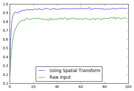
画图比较正确率与训练次数

plt.plot(l_acc, label="Using Spatial Transform")
plt.plot(l_acc_F, label="Raw input")
plt.legend(loc=8)

可见 Spatial Transform 确实可以提升分类的正确率。

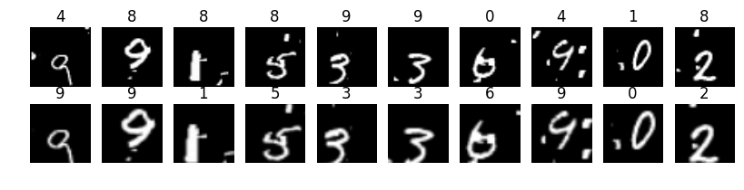
最后，我们专门提出来直接分类分错、Spatial Transform 后分类正确的数字。上面一行是直接预测的结果（错误），下面一行是转换后分类的结果：



通过 Spatial Transform，我们确实可以强化数据的特征，增加数据分类的准确性。

此外，Spatial Transform 除了可以识别“草书”字体的手写数字，同样在交通标志分类中表现优异，通过Spatial Transform 元件与 LeNet-5 网络的组合，Yann LeCun团队实现了42种交通标志分类99.1%准确性（笔者直接用LeNet-5发现准确率只有87%左右），文章地址Traffic
Sign Recognition with Multi-Scale Convolutional Networks



目前腾讯云 GPU 服务器已经在5月27日盛大公测，本章代码也可以用较小的数据量、较低的nb_epoch在普通云服务器上尝试一下，但是随着处理运算量越来越大，必须租用 云GPU服务器 才可以快速算出结果。服务器的租用方式、价格，详情请见 腾讯云
GPU 云服务器今日全量上线！