cs231n的第一次作业2层神经网络

一个小测试，测试写的函数对不对

首先是初始化

input_size = 4
hidden_size = 10
num_classes = 3
num_inputs = 5

def init_toy_model():
np.random.seed(0)
return TwoLayerNet(input_size, hidden_size, num_classes, std=1e-1)

def init_toy_data():
np.random.seed(1)
X = 10 * np.random.randn(num_inputs, input_size)
y = np.array([0, 1, 2, 2, 1])
return X, y

net = init_toy_model()
X, y = init_toy_data()
print X.shape, y.shape

初始化

class TwoLayerNet(object):
def __init__(self, input_size, hidden_size, output_size, std=1e-4):
"""
Initialize the model. Weights are initialized to small random values and
biases are initialized to zero. Weights and biases are stored in the
variable self.params, which is a dictionary with the following keys:

W1: First layer weights; has shape (D, H)
b1: First layer biases; has shape (H,)
W2: Second layer weights; has shape (H, C)
b2: Second layer biases; has shape (C,)

Inputs:
- input_size: The dimension D of the input data.
- hidden_size: The number of neurons H in the hidden layer.
- output_size: The number of classes C.
"""
self.params = {}
self.params['W1'] = std * np.random.randn(input_size, hidden_size)
self.params['b1'] = np.zeros(hidden_size)
self.params['W2'] = std * np.random.randn(hidden_size, output_size)
self.params['b2'] = np.zeros(output_size)

对于W1的维数，即将输入样本的个数每个分配一个权重，最后输出相当于是hidden_size个分数，然后这些分数和激活函数相比较，b1应该是比较的阈值吧（自己觉得），有些分数就不会起作用。这样得
4000
到处理后的分数，在与W2相乘，与激活函数相比较，可以看到，W2输出是output_size，也就是说，输出的分数和类别数一样，即最终的分数。这里初始化这四个参数的意思大概就是这样子。

X的大小X.shape = (5, 4)

y的大小y.shape = (5, )

net.params[‘W1’].shape = (4, 10)

net.params[‘b1’].shape = (10, )

net.params[‘W2’].shape = (10, 3)

net.params[‘b2’].shape = (3, )

知道了维数关系，也就清楚了是 X*W 而不是 W*X，这个按实际去写，不要硬记。

计算loss和grad

def loss(self, X, y=None, reg=0.0):
"""
Compute the loss and gradients for a two layer fully connected neural network.

Inputs:
- X: Input data of shape (N, D). Each X[i] is a training sample.
- y: Vector of training labels. y[i] is the label for X[i], and each y[i] is
an integer in the range 0 <= y[i] < C. This parameter is optional; if it
is not passed then we only return scores, and if it is passed then we
instead return the loss and gradients.
- reg: Regularization strength.

Returns:
If y is None, return a matrix scores of shape (N, C) where scores[i, c] is
the score for class c on input X[i].

If y is not None, instead return a tuple of:
- loss: Loss (data loss and regularization loss) for this batch of training
samples.
- grads: Dictionary mapping parameter names to gradients of those parameters
with respect to the loss function; has the same keys as self.params.
"""
# Unpack variables from the params dictionary
W1, b1 = self.params['W1'], self.params['b1']
W2, b2 = self.params['W2'], self.params['b2']
N, D = X.shape

# Compute the forward pass
scores = None
# Perform the forward pass, computing the class scores for the input.
# score.shape (N, C).
h_output = np.maximum(0, X.dot(W1) + b1)  # (N,D) * (D,H) = (N,H)
scores = h_output.dot(W2) + b2

# If the targets are not given then jump out, we're done
if y is None:
return scores

# Compute the loss
loss = None

#Finish the forward pass, and compute the loss.
shift_scores = scores - np.max(scores, axis=1).reshape(-1, 1)
softmax_output = np.exp(shift_scores) / np.sum(np.exp(shift_scores), axis=1).reshape(-1, 1)
loss = -np.sum(np.log(softmax_output[range(N), list(y)]))
loss /= N
loss += 0.5 * reg * (np.sum(W1 * W1) + np.sum(W2 * W2))

# Backward pass: compute gradients
grads = {}

# Compute the backward pass, computing the derivatives of the weights #
# and biases. Store the results in the grads dictionary. For example,       #
# grads['W1'] should store the gradient on W1, and be a matrix of same size #
dscores = softmax_output.copy()
dscores[range(N), list(y)] -= 1
dscores /= N
grads['W2'] = h_output.T.dot(dscores) + reg * W2
grads['b2'] = np.sum(dscores, axis=0)

dh = dscores.dot(W2.T)
dh_ReLu = (h_output > 0) * dh
grads['W1'] = X.T.dot(dh_ReLu) + reg * W1
grads['b1'] = np.sum(dh_ReLu, axis=0)
return loss, grads

得分scores的计算,由之前权重W和输入X的shape可知，

h_output = np.maximum(0, X.dot(W1) + b1) #第一层网络，激活函数为max().

scores = h_output.dot(W2) + b2 #第二层网络，最后得到每个样本的分数

损失loss的计算，这里用的是softmax的损失函数，所以，要先减去最大值，归一化，达到数值稳定。最后取了平均并且加了1/2的正则化项。

shift_scores = scores - np.max(scores, axis=1).reshape(-1, 1) #为了数值稳定

softmax_output = np.exp(shift_scores) / np.sum(np.exp(shift_scores), axis=1).reshape(-1, 1)#算了所有的 分数/sum

loss = -np.sum(np.log(softmax_output[range(N), list(y)])) #损失是正确的分类的分数/sum

loss /= N #compute average

loss += 0.5 * reg * (np.sum(W1 * W1) + np.sum(W2 * W2))#加正则项，这些可以参考之前的softmax

对于梯度的计算，对分类正确的Wyi分类器求导要多一个-Xi（具体求导可以参考上篇softmax博客），所以这是下面第三行-1的原因。但是为什么没有乘以X呢(⊙o⊙)?，求解答

反向传播计算线路参考图



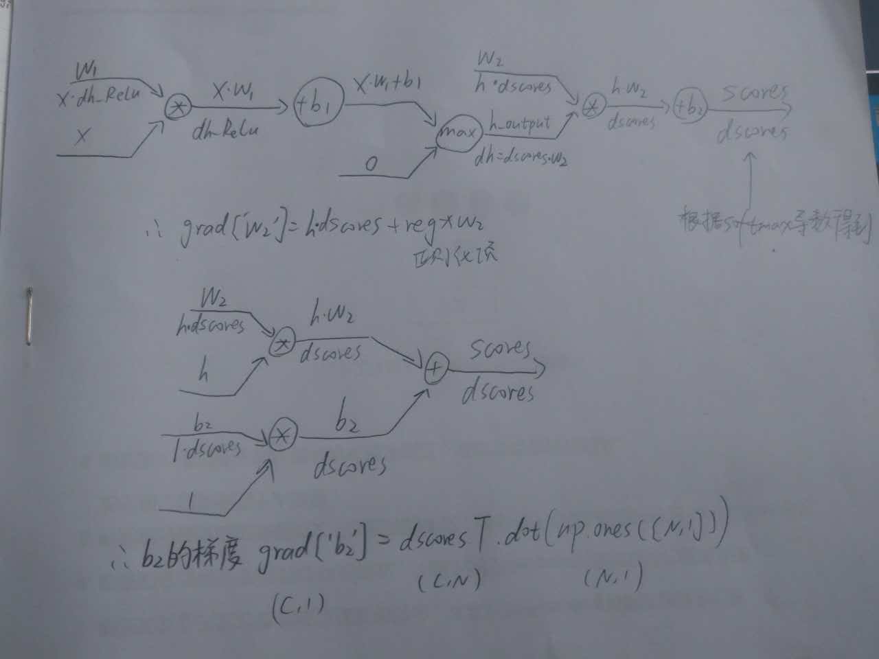
具体对应的代码

grads = {}
dscores = softmax_output.copy()
dscores[range(N), list(y)] -= 1
dscores /= N
grads['W2'] = h_output.T.dot(dscores) + reg * W2
grads['b2'] = np.sum(dscores, axis=0)
dh = dscores.dot(W2.T)
dh_ReLu = (h_output > 0) * dh
grads['W1'] = X.T.dot(dh_ReLu) + reg * W1
grads['b1'] = np.sum(dh_ReLu, axis=0)

最后的测试结果，和提供的正确数据几乎一致

W1 max relative error: 3.561318e-09

W2 max relative error: 3.440708e-09

b2 max relative error: 4.447625e-11

b1 max relative error: 2.738421e-09

训练

def train(self, X, y, X_val, y_val,
learning_rate=1e-3, learning_rate_decay=0.95,
reg=1e-5, num_iters=100,
batch_size=200, verbose=False):
"""
Train this neural network using stochastic gradient descent.

Inputs:
- X: A numpy array of shape (N, D) giving training data.
- y: A numpy array f shape (N,) giving training labels; y[i] = c means that
X[i] has label c, where 0 <= c < C.
- X_val: A numpy array of shape (N_val, D) giving validation data.
- y_val: A numpy array of shape (N_val,) giving validation labels.
- learning_rate: Scalar giving learning rate for optimization.
- learning_rate_decay: Scalar giving factor used to decay the learning rate
after each epoch.
- reg: Scalar giving regularization strength.
- num_iters: Number of steps to take when optimizing.
- batch_size: Number of training examples to use per step.
- verbose: boolean; if true print progress during optimization.
"""
num_train = X.shape[0]
iterations_per_epoch = max(num_train / batch_size, 1)

# Use SGD to optimize the parameters in self.model
loss_history = []
train_acc_history = []
val_acc_history = []

for it in xrange(num_iters):
X_batch = None
y_batch = None

# Create a random minibatch of training data and labels, storing  #
# them in X_batch and y_batch respectively.                             #

idx = np.random.choice(num_train, batch_size, replace=True)
X_batch = X[idx]
y_batch = y[idx]

# Compute loss and gradients using the current minibatch
loss, grads = self.loss(X_batch, y=y_batch, reg=reg)
loss_history.append(loss)

# Use the gradients in the grads dictionary to update the         #
# parameters of the network (stored in the dictionary self.params)      #
# using stochastic gradient descent. You'll need to use the gradients   #
# stored in the grads dictionary defined above.                         #
self.params['W2'] += - learning_rate * grads['W2']
self.params['b2'] += - learning_rate * grads['b2']
self.params['W1'] += - learning_rate * grads['W1']
self.params['b1'] += - learning_rate * grads['b1']

if verbose and it % 100 == 0:
print 'iteration %d / %d: loss %f' % (it, num_iters, loss)

# Every epoch, check train and val accuracy and decay learning rate.
if it % iterations_per_epoch == 0:
# Check accuracy
train_acc = (self.predict(X_batch) == y_batch).mean()
val_acc = (self.predict(X_val) == y_val).mean()
train_acc_history.append(train_acc)
val_acc_history.append(val_acc)

# Decay learning rate
learning_rate *= learning_rate_decay

return {
'loss_history': loss_history,
'train_acc_history': train_acc_history,
'val_acc_history': val_acc_history,
}

训练基本和之前的softmax和svm一样，取小样本，计算损失和梯度，用SGD更新W和b（在svm中，W增加了一列，放b）。

最后的几句代码，计算了预测准确率，并且学习率在不停的减小。

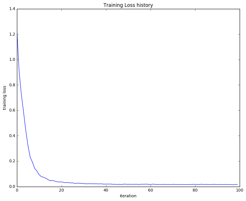
画出loss_history与迭代次数的曲线，可以看到20次后loss基本不变。

开始用CIFAR10数据实战

测试小例子很成功呀，是时候开始用CIFAR10数据来实验。

input_size = 32 * 32 * 3
hidden_size = 50
num_classes = 10
net = TwoLayerNet(input_size, hidden_size, num_classes)

# Train the network
stats = net.train(X_train, y_train, X_val, y_val,
num_iters=1000, batch_size=200,
learning_rate=1e-4, learning_rate_decay=0.95,
reg=0.5, verbose=True)

# Predict on the validation set
val_acc = (net.predict(X_val) == y_val).mean()
print 'Validation accuracy: ', val_acc

输出结果

iteration 0 / 1000: loss 2.302954

iteration 100 / 1000: loss 2.302550

iteration 200 / 1000: loss 2.297648

iteration 300 / 1000: loss 2.259602

iteration 400 / 1000: loss 2.204170

iteration 500 / 1000: loss 2.118565

iteration 600 / 1000: loss 2.051535

iteration 700 / 1000: loss 1.988466

iteration 800 / 1000: loss 2.006591

iteration 900 / 1000: loss 1.951473

Validation accuracy: 0.287

训练集的准确率只有28.7%，不太理想呀



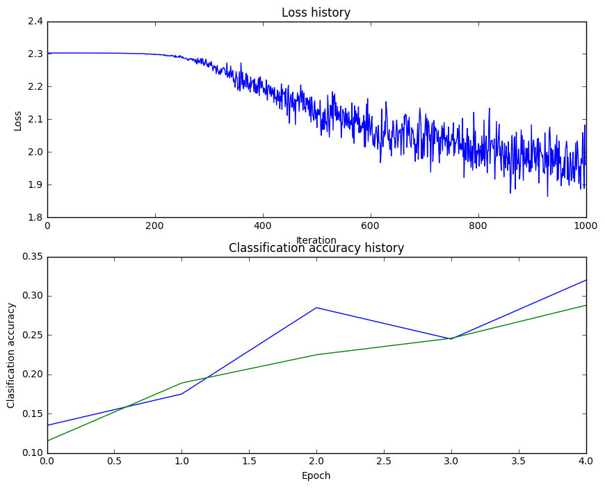
蓝线为 train_acc_history，绿线为 val_acc_history

hidden_size = [75, 100, 12
a1d8
5]

learning_rates = np.array([0.7, 0.8, 0.9, 1, 1.1])*1e-3

regularization_strengths = [0.75, 1, 1.25]

hs 100 lr 1.100000e-03 reg 7.500000e-01 val accuracy: 0.502000

best validation accuracy achieved during cross-validation: 0.502000

用了三层for循环，硬生生找了三个较好的参数，准确率达到了50.2%

hint里提示用PCA降维，adding dropout, 或者adding features to the solver来到达更好的效果，这些先放着以后试吧（加粗防忘记）

参考

(对了如果想保存网页内容，可以用chrome浏览器，右键打印，保存为pdf，可以选择保存的页数，再打印出来看，对着电脑看眼睛吃不消了)

知乎翻译https://zhuanlan.zhihu.com/p/21407711?refer=intelligentunit

建议看看课件和视频https://www.youtube.com/watch?v=GZTvxoSHZIo&t=3093s