examples - visualizing time series data and geographic data using python

In [1]:

import pandas as pd

In [2]:

bird_data = pd.read_csv('./bird_tracking.csv')

In [3]:

bird_data.head()

Out[3]:

	altitude	date_time	device_info_serial	direction	latitude	longitude	speed_2d	bird_name
0	71	2013-08-15 00:18:08+00	851	-150.469753	49.419859	2.120733	0.150000	Eric
1	68	2013-08-15 00:48:07+00	851	-136.151141	49.419880	2.120746	2.438360	Eric
2	68	2013-08-15 01:17:58+00	851	160.797477	49.420310	2.120885	0.596657	Eric
3	73	2013-08-15 01:47:51+00	851	32.769360	49.420359	2.120859	0.310161	Eric
4	69	2013-08-15 02:17:42+00	851	45.191230	49.420331	2.120887	0.193132	Eric

In [4]:

bird_data.info()

<class 'pandas.core.frame.DataFrame'>
RangeIndex: 61920 entries, 0 to 61919
Data columns (total 8 columns):
altitude              61920 non-null int64
date_time             61920 non-null object
device_info_serial    61920 non-null int64
direction             61477 non-null float64
latitude              61920 non-null float64
longitude             61920 non-null float64
speed_2d              61477 non-null float64
bird_name             61920 non-null object
dtypes: float64(4), int64(2), object(2)
memory usage: 3.8+ MB

In [5]:

import matplotlib.pyplot as plt
import numpy as np

In [6]:

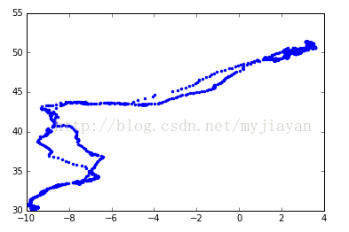
idx = bird_data.bird_name == 'Eric'

In [7]:

eric_x, eric_y = bird_data.longitude[idx], bird_data.latitude[idx]

In [8]:

plt.figure(figsize=(7,7))

Out[8]:

<matplotlib.figure.Figure at 0x8c60630>

In [9]:

%matplotlib inline
plt.plot(eric_x,eric_y,'.')

Out[9]:

[<matplotlib.lines.Line2D at 0x5f3def0>]

In [10]:

all_bird_names = pd.unique(bird_data.bird_name)

In [11]:

all_bird_names

Out[11]:

array(['Eric', 'Nico', 'Sanne'], dtype=object)

In [12]:

plt.figure(figsize=(7,7))for name in all_bird_names:
idx = bird_data.bird_name == name
x, y = bird_data.longitude[idx], bird_data.latitude[idx]
plt.plot(x,y,'.',label=name)
plt.xlabel('Longitude')
plt.ylabel('Latitude')
plt.legend(loc='lower right')

Out[12]:

<matplotlib.legend.Legend at 0x8dd76d8>

looking at the speed of bird Eric¶

In [13]:

idx = bird_data.bird_name == 'Eric'

In [14]:

speed = bird_data.speed_2d[idx]

In [15]:

any(np.isnan(speed)) # or np.isnan(speed).any()

Out[15]:

True

There must be some value is not a numerical value.We need to pay attention.

In [16]:

np.sum(np.isnan(speed))

Out[16]:

85

There are 85 values that are not numerical values.

In [17]:

ind = np.isnan(speed)

In [18]:

plt.hist(speed[~ind])

Out[18]:

(array([  1.77320000e+04,   1.50200000e+03,   3.69000000e+02,
7.80000000e+01,   1.20000000e+01,   7.00000000e+00,
3.00000000e+00,   2.00000000e+00,   3.00000000e+00,
2.00000000e+00]),
array([  0.        ,   6.34880658,  12.69761316,  19.04641974,
25.39522632,  31.7440329 ,  38.09283948,  44.44164607,
50.79045265,  57.13925923,  63.48806581]),
<a list of 10 Patch objects>)

In [19]:

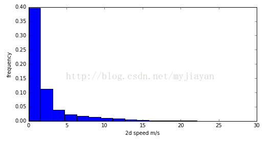
plt.figure(figsize=(8,4))
plt.hist(speed[~ind], bins=np.linspace(0,30,20),normed=True)
plt.xlabel('2d speed m/s')
plt.ylabel('frequency')

Out[19]:

<matplotlib.text.Text at 0x92eada0>

using pandas to plot histogram of speed¶

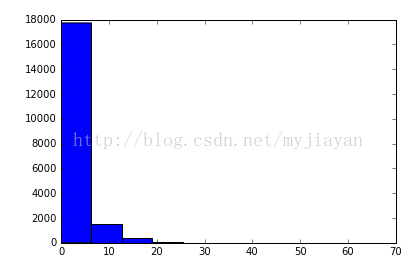
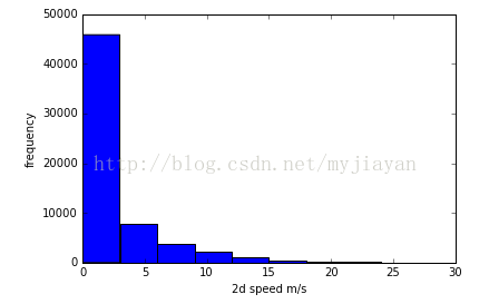
In [20]:

bird_data.speed_2d.plot(kind='hist',range=[0,30])
plt.xlabel('2d speed m/s')
plt.ylabel('frequency')

Out[20]:

<matplotlib.text.Text at 0x9906518>

dealing with dates¶

In [21]:

import datetime

In [22]:

datetime.datetime.today()

Out[22]:

datetime.datetime(2016, 12, 9, 15, 42, 19, 185079)

In [23]:

time1 = datetime.datetime.today()

In [24]:

time2 = datetime.datetime.today()

In [25]:

time2 - time1

Out[25]:

datetime.timedelta(0, 1, 729099)

In [26]:

date_str = bird_data.date_time[0]

In [27]:

date_str

Out[27]:

'2013-08-15 00:18:08+00'

In [28]:

date_str = date_str[:-3]

In [29]:

date_str

Out[29]:

'2013-08-15 00:18:08'

In [30]:

datetime.datetime.strptime(date_str, "%Y-%m-%d %H:%M:%S")

Out[30]:

datetime.datetime(2013, 8, 15, 0, 18, 8)

In [31]:

def date_str2_date(date_str):
return datetime.datetime.strptime(date_str[:-3], "%Y-%m-%d %H:%M:%S")

In [32]:

timestamp = bird_data.date_time.apply(date_str2_date)

In [33]:

timestamp[:10]

Out[33]:

0   2013-08-15 00:18:08
1   2013-08-15 00:48:07
2   2013-08-15 01:17:58
3   2013-08-15 01:47:51
4   2013-08-15 02:17:42
5   2013-08-15 02:47:38
6   2013-08-15 03:02:33
7   2013-08-15 03:17:27
8   2013-08-15 03:32:35
9   2013-08-15 03:47:48
Name: date_time, dtype: datetime64[ns]

In [34]:

bird_data['timestamp'] = timestamp

In [35]:

bird_data.columns

Out[35]:

Index(['altitude', 'date_time', 'device_info_serial', 'direction', 'latitude',
'longitude', 'speed_2d', 'bird_name', 'timestamp'],
dtype='object')

In [36]:

time = bird_data.timestamp[idx] # Eric

In [37]:

elasped_time = time - time[0]

In [38]:

elasped_time[:10]

Out[38]:

0   00:00:00
1   00:29:59
2   00:59:50
3   01:29:43
4   01:59:34
5   02:29:30
6   02:44:25
7   02:59:19
8   03:14:27
9   03:29:40
Name: timestamp, dtype: timedelta64[ns]

In [39]:

elasped_time[1000] / datetime.timedelta(days=1)

Out[39]:

12.084722222222222

In [40]:

elasped_time[1000] / datetime.timedelta(hours=1)

Out[40]:

290.03333333333336

In [41]:

elasped_days = elasped_time / datetime.timedelta(days=1)

In [42]:

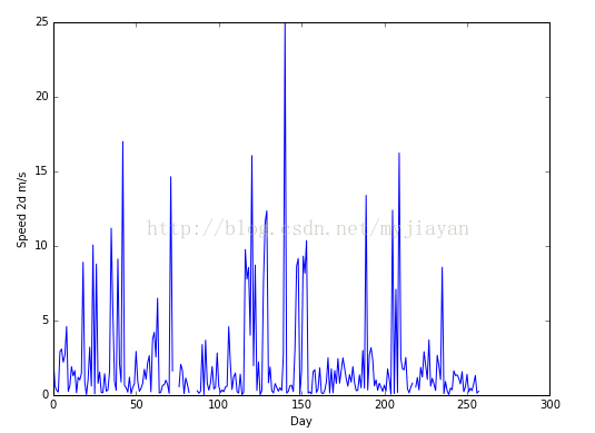
next_day = 1
ins = []
daily_mean_speed = []
for i,t in enumerate(elasped_days):
if t < next_day:
ins.append(next_day)
else:
daily_mean_speed.append(np.mean(bird_data.speed_2d[ins]))
next_day += 1
ins = []

In [43]:

plt.figure(figsize=(8,6))
plt.plot(daily_mean_speed)
plt.xlabel('Day')
plt.ylabel('Speed 2d m/s')

Out[43]:

<matplotlib.text.Text at 0x99aed68>

In [44]:

idx = bird_data.bird_name == 'Sanne'

In [45]:

bird_data.columns

Out[45]:

Index(['altitude', 'date_time', 'device_info_serial', 'direction', 'latitude',
'longitude', 'speed_2d', 'bird_name', 'timestamp'],
dtype='object')

In [46]:

bird_data.date_time[idx]

Out[46]:

40916    2013-08-15 00:01:08+00
40917    2013-08-15 00:31:00+00
40918    2013-08-15 01:01:19+00
40919    2013-08-15 01:31:38+00
40920    2013-08-15 02:01:24+00
40921    2013-08-15 02:31:18+00
40922    2013-08-15 03:00:54+00
40923    2013-08-15 03:15:57+00
40924    2013-08-15 03:31:13+00
40925    2013-08-15 03:46:28+00
40926    2013-08-15 04:01:56+00
40927    2013-08-15 04:16:55+00
40928    2013-08-15 04:31:54+00
40929    2013-08-15 04:47:08+00
40930    2013-08-15 05:02:15+00
40931    2013-08-15 05:17:08+00
40932    2013-08-15 05:32:04+00
40933    2013-08-15 05:46:58+00
40934    2013-08-15 06:01:55+00
40935    2013-08-15 06:16:50+00
40936    2013-08-15 06:31:47+00
40937    2013-08-15 06:46:43+00
40938    2013-08-15 07:01:42+00
40939    2013-08-15 07:16:44+00
40940    2013-08-15 07:31:59+00
40941    2013-08-15 07:47:01+00
40942    2013-08-15 08:02:53+00
40943    2013-08-15 08:17:56+00
40944    2013-08-15 08:32:50+00
40945    2013-08-15 08:48:01+00
...
61890    2014-04-30 13:55:30+00
61891    2014-04-30 14:26:08+00
61892    2014-04-30 14:41:56+00
61893    2014-04-30 15:12:33+00
61894    2014-04-30 15:43:02+00
61895    2014-04-30 16:13:16+00
61896    2014-04-30 16:28:04+00
61897    2014-04-30 16:43:05+00
61898    2014-04-30 16:58:01+00
61899    2014-04-30 17:28:02+00
61900    2014-04-30 17:43:39+00
61901    2014-04-30 17:58:29+00
61902    2014-04-30 18:15:05+00
61903    2014-04-30 18:29:57+00
61904    2014-04-30 18:44:53+00
61905    2014-04-30 18:59:49+00
61906    2014-04-30 19:14:51+00
61907    2014-04-30 19:29:44+00
61908    2014-04-30 19:44:38+00
61909    2014-04-30 19:59:35+00
61910    2014-04-30 20:14:32+00
61911    2014-04-30 20:29:56+00
61912    2014-04-30 20:44:56+00
61913    2014-04-30 20:59:52+00
61914    2014-04-30 21:29:45+00
61915    2014-04-30 22:00:08+00
61916    2014-04-30 22:29:57+00
61917    2014-04-30 22:59:52+00
61918    2014-04-30 23:29:43+00
61919    2014-04-30 23:59:34+00
Name: date_time, dtype: object

In [48]:

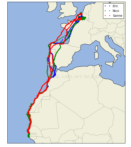
import cartopy.crs as ccrs
import cartopy.feature as cfeature

In [49]:

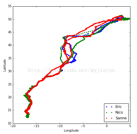
proj = ccrs.Mercator()
plt.figure(figsize=(10,10))
ax = plt.axes(projection=proj)
ax.set_extent((-25.0,20.0,52.0,10.0))
ax.add_feature(cfeature.LAND)
ax.add_feature(cfeature.OCEAN)
ax.add_feature(cfeature.COASTLINE)
ax.add_feature(cfeature.BORDERS, linestyle=':')
for name in all_bird_names:
idx = bird_data.bird_name == name
x, y = bird_data.longitude[idx], bird_data.latitude[idx]
ax.plot(x,y, '.',transform=ccrs.Geodetic(), label=name)
plt.legend(loc='best')

Out[49]:

<matplotlib.legend.Legend at 0xaf8beb8>

C:\Anaconda3\lib\site-packages\cartopy\io\__init__.py:264: DownloadWarning: Downloading: http://naciscdn.org/naturalearth/110m/physical/ne_110m_land.zip warnings.warn('Downloading: {}'.format(url), DownloadWarning)
C:\Anaconda3\lib\site-packages\cartopy\io\__init__.py:264: DownloadWarning: Downloading: http://naciscdn.org/naturalearth/110m/physical/ne_110m_ocean.zip warnings.warn('Downloading: {}'.format(url), DownloadWarning)
C:\Anaconda3\lib\site-packages\cartopy\io\__init__.py:264: DownloadWarning: Downloading: http://naciscdn.org/naturalearth/110m/physical/ne_110m_coastline.zip warnings.warn('Downloading: {}'.format(url), DownloadWarning)
C:\Anaconda3\lib\site-packages\cartopy\io\__init__.py:264: DownloadWarning: Downloading: http://naciscdn.org/naturalearth/110m/cultural/ne_110m_admin_0_boundary_lines_land.zip warnings.warn('Downloading: {}'.format(url), DownloadWarning)

In [53]:

grouped_birds = bird_data.groupby("bird_name")

In [54]:

bird_data.date_time = pd.to_datetime(bird_data.date_time)

In [57]:

bird_data["date"] = bird_data.date_time.dt.date

In [65]:

grouped_bydates = bird_data.groupby(['bird_name','date'])

In [66]:

grouped_birdday = bird_data.groupby(['bird_name','date'])

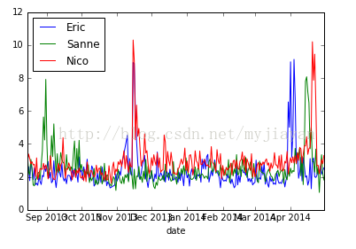
In [67]:

eric_daily_speed  = grouped_bydates.speed_2d.mean()["Eric"]
sanne_daily_speed = grouped_bydates.speed_2d.mean()["Sanne"]
nico_daily_speed  = grouped_bydates.speed_2d.mean()["Nico"]

eric_daily_speed.plot(label="Eric")
sanne_daily_speed.plot(label="Sanne")
nico_daily_speed.plot(label="Nico")
plt.legend(loc="best")

Out[67]:

<matplotlib.legend.Legend at 0xaf92128>