DeepLearnToolbox及CNN代码实现
2016-05-02 19:18
253 查看
使用的代码:DeepLearnToolbox
,下载地址:点击打开,感谢该toolbox的作者
==========================================================================================
今天是CNN的内容啦,CNN讲起来有些纠结,你可以事先看看convolution和pooling(subsampling),还有这篇:tornadomeet的博文
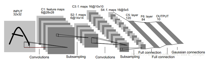
下面是那张经典的图:
======================================================================================================
打开\tests\test_example_CNN.m一观
[cpp] view
plain copy


cnn.layers = {
struct('type', 'i') %input layer
struct('type', 'c', 'outputmaps', 6, 'kernelsize', 5) %convolution layer
struct('type', 's', 'scale', 2) %sub sampling layer
struct('type', 'c', 'outputmaps', 12, 'kernelsize', 5) %convolution layer
struct('type', 's', 'scale', 2) %subsampling layer
};
cnn = cnnsetup(cnn, train_x, train_y); //here!!!
opts.alpha = 1;
opts.batchsize = 50;
opts.numepochs = 1;
cnn = cnntrain(cnn, train_x, train_y, opts); //here!!!
似乎这次要复杂了一些啊,首先是layer,有三种,i是input,c是convolution,s是subsampling
'c'的outputmaps是convolution之后有多少张图,比如上(最上那张经典的))第一层convolution之后就有六个特征图
'c'的kernelsize 其实就是用来convolution的patch是多大
's'的scale就是pooling的size为scale*scale的区域
接下来似乎就是常规思路了,cnnsetup()和cnntrain()啦,我们来看代码
主要是一些参数的作用的解释,详细的参看代码里的注释啊
[cpp] view
plain copy
function net = cnnsetup(net, x, y)
inputmaps = 1;
mapsize = size(squeeze(x(:, :, 1)));
//尤其注意这几个循环的参数的设定
//numel(net.layers) 表示有多少层
for l = 1 : numel(net.layers) // layer
if strcmp(net.layers{l}.type, 's')
mapsize = mapsize / net.layers{l}.scale;
//subsampling层的mapsize,最开始mapsize是每张图的大小28*28(这是第一次卷积后的结果,卷积前是32*32)
//这里除以scale,就是pooling之后图的大小,这里为14*14
assert(all(floor(mapsize)==mapsize), ['Layer ' num2str(l) ' size must be integer. Actual: ' num2str(mapsize)]);
for j = 1 : inputmaps //inputmap就是上一层有多少张特征图,通过初始化为1然后依层更新得到
net.layers{l}.b{j} = 0;
end
end
if strcmp(net.layers{l}.type, 'c')
mapsize = mapsize - net.layers{l}.kernelsize + 1;
//这里的mapsize可以参见UFLDL里面的那张图下面的解释
fan_out = net.layers{l}.outputmaps * net.layers{l}.kernelsize ^ 2;
//隐藏层的大小,是一个(后层特征图数量)*(用来卷积的patch图的大小)
for j = 1 : net.layers{l}.outputmaps // output map
fan_in = inputmaps * net.layers{l}.kernelsize ^ 2;
//对于每一个后层特征图,有多少个参数链到前层
for i = 1 : inputmaps // input map
net.layers{l}.k{i}{j} = (rand(net.layers{l}.kernelsize) - 0.5) * 2 * sqrt(6 / (fan_in + fan_out));
end
net.layers{l}.b{j} = 0;
end
inputmaps = net.layers{l}.outputmaps;
end
end
// 'onum' is the number of labels, that's why it is calculated using size(y, 1). If you have 20 labels so the output of the network will be 20 neurons.
// 'fvnum' is the number of output neurons at the last layer, the layer just before the output layer.
// 'ffb' is the biases of the output neurons.
// 'ffW' is the weights between the last layer and the output neurons. Note that the last layer is fully connected to the output layer, that's why the size of the weights is (onum * fvnum)
fvnum = prod(mapsize) * inputmaps;
onum = size(y, 1);
//这里是最后一层神经网络的设定
net.ffb = zeros(onum, 1);
net.ffW = (rand(onum, fvnum) - 0.5) * 2 * sqrt(6 / (onum + fvnum));
end
[cpp] view
plain copy
net = cnnff(net, batch_x);
net = cnnbp(net, batch_y);
net = cnnapplygrads(net, opts);
cnntrain是用back propagation来计算gradient的,我们一次来看这三个函数:
这部分计算还比较简单,可以说是有迹可循,大家最好看看tornadomeet的博文的步骤,说得比较清楚
[cpp] view
plain copy
function net = cnnff(net, x)
n = numel(net.layers);
net.layers{1}.a{1} = x;
inputmaps = 1;
for l = 2 : n // for each layer
if strcmp(net.layers{l}.type, 'c')
// !!below can probably be handled by insane matrix operations
for j = 1 : net.layers{l}.outputmaps // for each output map
// create temp output map
z = zeros(size(net.layers{l - 1}.a{1}) - [net.layers{l}.kernelsize - 1 net.layers{l}.kernelsize - 1 0]);
for i = 1 : inputmaps // for each input map
// convolve with corresponding kernel and add to temp output map
// 做卷积,参考UFLDL,这里是对每一个input的特征图做一次卷积,再加起来
z = z + convn(net.layers{l - 1}.a{i}, net.layers{l}.k{i}{j}, 'valid');
end
// add bias, pass through nonlinearity
// 加入bias
net.layers{l}.a{j} = sigm(z + net.layers{l}.b{j});
end
// set number of input maps to this layers number of outputmaps
inputmaps = net.layers{l}.outputmaps;
elseif strcmp(net.layers{l}.type, 's')
// downsample
for j = 1 : inputmaps
//这里有点绕绕的,它是新建了一个patch来做卷积,但我们要的是pooling,所以它跳着把结果读出来,步长为scale
//这里做的是mean-pooling
z = convn(net.layers{l - 1}.a{j}, ones(net.layers{l}.scale) / (net.layers{l}.scale ^ 2), 'valid'); // !! replace with variable
net.layers{l}.a{j} = z(1 : net.layers{l}.scale : end, 1 : net.layers{l}.scale : end, :);
end
end
end
// 收纳到一个vector里面,方便后面用~~
// concatenate all end layer feature maps into vector
net.fv = [];
for j = 1 : numel(net.layers{n}.a)
sa = size(net.layers{n}.a{j});
net.fv = [net.fv; reshape(net.layers{n}.a{j}, sa(1) * sa(2), sa(3))];
end
// 最后一层的perceptrons,数据识别的结果
net.o = sigm(net.ffW * net.fv + repmat(net.ffb, 1, size(net.fv, 2)));
end
这个就哭了,代码有些纠结,不得已又找资料看啊,《Notes on Convolutional Neural Networks》要好一些
只是这个toolbox的代码和《Notes on Convolutional Neural Networks》里有些不一样的是这个toolbox在subsampling(也就是pooling层)没有加sigmoid激活函数,只是单纯地pooling了一下,所以这地方还需仔细辨别,这个toolbox里的subsampling是不用计算gradient的,而在Notes里是计算了的
还有这个toolbox没有Combinations of Feature Maps,也就是tornadomeet的博文里这张表格:
具体就去看看上面这篇论文吧

然后就看代码吧:
[cpp] view
plain copy
function net = cnnbp(net, y)
n = numel(net.layers);
// error
net.e = net.o - y;
// loss function
net.L = 1/2* sum(net.e(:) .^ 2) / size(net.e, 2);
//从最后一层的error倒推回来deltas
//和神经网络的bp有些类似
//// backprop deltas
net.od = net.e .* (net.o .* (1 - net.o)); // output delta
net.fvd = (net.ffW' * net.od); // feature vector delta
if strcmp(net.layers{n}.type, 'c') // only conv layers has sigm function
net.fvd = net.fvd .* (net.fv .* (1 - net.fv));
end
//和神经网络类似,参看神经网络的bp
// reshape feature vector deltas into output map style
sa = size(net.layers{n}.a{1});
fvnum = sa(1) * sa(2);
for j = 1 : numel(net.layers{n}.a)
net.layers{n}.d{j} = reshape(net.fvd(((j - 1) * fvnum + 1) : j * fvnum, :), sa(1), sa(2), sa(3));
end
//这是算delta的步骤
//这部分的计算参看Notes on Convolutional Neural Networks,其中的变化有些复杂
//和这篇文章里稍微有些不一样的是这个toolbox在subsampling(也就是pooling层)没有加sigmoid激活函数
//所以这地方还需仔细辨别
//这这个toolbox里的subsampling是不用计算gradient的,而在上面那篇note里是计算了的
for l = (n - 1) : -1 : 1
if strcmp(net.layers{l}.type, 'c')
for j = 1 : numel(net.layers{l}.a)
net.layers{l}.d{j} = net.layers{l}.a{j} .* (1 - net.layers{l}.a{j}) .* (expand(net.layers{l + 1}.d{j}, [net.layers{l + 1}.scale net.layers{l + 1}.scale 1]) / net.layers{l + 1}.scale ^ 2);
end
elseif strcmp(net.layers{l}.type, 's')
for i = 1 : numel(net.layers{l}.a)
z = zeros(size(net.layers{l}.a{1}));
for j = 1 : numel(net.layers{l + 1}.a)
z = z + convn(net.layers{l + 1}.d{j}, rot180(net.layers{l + 1}.k{i}{j}), 'full');
end
net.layers{l}.d{i} = z;
end
end
end
//参见paper,注意这里只计算了'c'层的gradient,因为只有这层有参数
//// calc gradients
for l = 2 : n
if strcmp(net.layers{l}.type, 'c')
for j = 1 : numel(net.layers{l}.a)
for i = 1 : numel(net.layers{l - 1}.a)
net.layers{l}.dk{i}{j} = convn(flipall(net.layers{l - 1}.a{i}), net.layers{l}.d{j}, 'valid') / size(net.layers{l}.d{j}, 3);
end
net.layers{l}.db{j} = sum(net.layers{l}.d{j}(:)) / size(net.layers{l}.d{j}, 3);
end
end
end
//最后一层perceptron的gradient的计算
net.dffW = net.od * (net.fv)' / size(net.od, 2);
net.dffb = mean(net.od, 2);
function X = rot180(X)
X = flipdim(flipdim(X, 1), 2);
end
end
这部分就轻松了,已经有grads了,依次进行梯度更新就好了
[cpp] view
plain copy
function net = cnnapplygrads(net, opts)
for l = 2 : numel(net.layers)
if strcmp(net.layers{l}.type, 'c')
for j = 1 : numel(net.layers{l}.a)
for ii = 1 : numel(net.layers{l - 1}.a)
net.layers{l}.k{ii}{j} = net.layers{l}.k{ii}{j} - opts.alpha * net.layers{l}.dk{ii}{j};
end
net.layers{l}.b{j} = net.layers{l}.b{j} - opts.alpha * net.layers{l}.db{j};
end
end
end
net.ffW = net.ffW - opts.alpha * net.dffW;
net.ffb = net.ffb - opts.alpha * net.dffb;
end
好吧,我们得知道最后结果怎么来啊
[cpp] view
plain copy
function [er, bad] = cnntest(net, x, y)
// feedforward
net = cnnff(net, x);
[~, h] = max(net.o);
[~, a] = max(y);
bad = find(h ~= a);
er = numel(bad) / size(y, 2);
end
就是这样~~cnnff一次后net.o就是结果
,下载地址:点击打开,感谢该toolbox的作者
==========================================================================================
今天是CNN的内容啦,CNN讲起来有些纠结,你可以事先看看convolution和pooling(subsampling),还有这篇:tornadomeet的博文
下面是那张经典的图:
======================================================================================================
打开\tests\test_example_CNN.m一观
[cpp] view
plain copy
cnn.layers = {
struct('type', 'i') %input layer
struct('type', 'c', 'outputmaps', 6, 'kernelsize', 5) %convolution layer
struct('type', 's', 'scale', 2) %sub sampling layer
struct('type', 'c', 'outputmaps', 12, 'kernelsize', 5) %convolution layer
struct('type', 's', 'scale', 2) %subsampling layer
};
cnn = cnnsetup(cnn, train_x, train_y); //here!!!
opts.alpha = 1;
opts.batchsize = 50;
opts.numepochs = 1;
cnn = cnntrain(cnn, train_x, train_y, opts); //here!!!
似乎这次要复杂了一些啊,首先是layer,有三种,i是input,c是convolution,s是subsampling
'c'的outputmaps是convolution之后有多少张图,比如上(最上那张经典的))第一层convolution之后就有六个特征图
'c'的kernelsize 其实就是用来convolution的patch是多大
's'的scale就是pooling的size为scale*scale的区域
接下来似乎就是常规思路了,cnnsetup()和cnntrain()啦,我们来看代码
\CNN\cnnsetup.m
主要是一些参数的作用的解释,详细的参看代码里的注释啊[cpp] view
plain copy
function net = cnnsetup(net, x, y)
inputmaps = 1;
mapsize = size(squeeze(x(:, :, 1)));
//尤其注意这几个循环的参数的设定
//numel(net.layers) 表示有多少层
for l = 1 : numel(net.layers) // layer
if strcmp(net.layers{l}.type, 's')
mapsize = mapsize / net.layers{l}.scale;
//subsampling层的mapsize,最开始mapsize是每张图的大小28*28(这是第一次卷积后的结果,卷积前是32*32)
//这里除以scale,就是pooling之后图的大小,这里为14*14
assert(all(floor(mapsize)==mapsize), ['Layer ' num2str(l) ' size must be integer. Actual: ' num2str(mapsize)]);
for j = 1 : inputmaps //inputmap就是上一层有多少张特征图,通过初始化为1然后依层更新得到
net.layers{l}.b{j} = 0;
end
end
if strcmp(net.layers{l}.type, 'c')
mapsize = mapsize - net.layers{l}.kernelsize + 1;
//这里的mapsize可以参见UFLDL里面的那张图下面的解释
fan_out = net.layers{l}.outputmaps * net.layers{l}.kernelsize ^ 2;
//隐藏层的大小,是一个(后层特征图数量)*(用来卷积的patch图的大小)
for j = 1 : net.layers{l}.outputmaps // output map
fan_in = inputmaps * net.layers{l}.kernelsize ^ 2;
//对于每一个后层特征图,有多少个参数链到前层
for i = 1 : inputmaps // input map
net.layers{l}.k{i}{j} = (rand(net.layers{l}.kernelsize) - 0.5) * 2 * sqrt(6 / (fan_in + fan_out));
end
net.layers{l}.b{j} = 0;
end
inputmaps = net.layers{l}.outputmaps;
end
end
// 'onum' is the number of labels, that's why it is calculated using size(y, 1). If you have 20 labels so the output of the network will be 20 neurons.
// 'fvnum' is the number of output neurons at the last layer, the layer just before the output layer.
// 'ffb' is the biases of the output neurons.
// 'ffW' is the weights between the last layer and the output neurons. Note that the last layer is fully connected to the output layer, that's why the size of the weights is (onum * fvnum)
fvnum = prod(mapsize) * inputmaps;
onum = size(y, 1);
//这里是最后一层神经网络的设定
net.ffb = zeros(onum, 1);
net.ffW = (rand(onum, fvnum) - 0.5) * 2 * sqrt(6 / (onum + fvnum));
end
\CNN\cnntrain.m
cnntrain就和nntrain是一个节奏了:[cpp] view
plain copy
net = cnnff(net, batch_x);
net = cnnbp(net, batch_y);
net = cnnapplygrads(net, opts);
cnntrain是用back propagation来计算gradient的,我们一次来看这三个函数:
cnnff.m
这部分计算还比较简单,可以说是有迹可循,大家最好看看tornadomeet的博文的步骤,说得比较清楚[cpp] view
plain copy
function net = cnnff(net, x)
n = numel(net.layers);
net.layers{1}.a{1} = x;
inputmaps = 1;
for l = 2 : n // for each layer
if strcmp(net.layers{l}.type, 'c')
// !!below can probably be handled by insane matrix operations
for j = 1 : net.layers{l}.outputmaps // for each output map
// create temp output map
z = zeros(size(net.layers{l - 1}.a{1}) - [net.layers{l}.kernelsize - 1 net.layers{l}.kernelsize - 1 0]);
for i = 1 : inputmaps // for each input map
// convolve with corresponding kernel and add to temp output map
// 做卷积,参考UFLDL,这里是对每一个input的特征图做一次卷积,再加起来
z = z + convn(net.layers{l - 1}.a{i}, net.layers{l}.k{i}{j}, 'valid');
end
// add bias, pass through nonlinearity
// 加入bias
net.layers{l}.a{j} = sigm(z + net.layers{l}.b{j});
end
// set number of input maps to this layers number of outputmaps
inputmaps = net.layers{l}.outputmaps;
elseif strcmp(net.layers{l}.type, 's')
// downsample
for j = 1 : inputmaps
//这里有点绕绕的,它是新建了一个patch来做卷积,但我们要的是pooling,所以它跳着把结果读出来,步长为scale
//这里做的是mean-pooling
z = convn(net.layers{l - 1}.a{j}, ones(net.layers{l}.scale) / (net.layers{l}.scale ^ 2), 'valid'); // !! replace with variable
net.layers{l}.a{j} = z(1 : net.layers{l}.scale : end, 1 : net.layers{l}.scale : end, :);
end
end
end
// 收纳到一个vector里面,方便后面用~~
// concatenate all end layer feature maps into vector
net.fv = [];
for j = 1 : numel(net.layers{n}.a)
sa = size(net.layers{n}.a{j});
net.fv = [net.fv; reshape(net.layers{n}.a{j}, sa(1) * sa(2), sa(3))];
end
// 最后一层的perceptrons,数据识别的结果
net.o = sigm(net.ffW * net.fv + repmat(net.ffb, 1, size(net.fv, 2)));
end
cnnbp.m
这个就哭了,代码有些纠结,不得已又找资料看啊,《Notes on Convolutional Neural Networks》要好一些只是这个toolbox的代码和《Notes on Convolutional Neural Networks》里有些不一样的是这个toolbox在subsampling(也就是pooling层)没有加sigmoid激活函数,只是单纯地pooling了一下,所以这地方还需仔细辨别,这个toolbox里的subsampling是不用计算gradient的,而在Notes里是计算了的
还有这个toolbox没有Combinations of Feature Maps,也就是tornadomeet的博文里这张表格:
具体就去看看上面这篇论文吧
然后就看代码吧:
[cpp] view
plain copy
function net = cnnbp(net, y)
n = numel(net.layers);
// error
net.e = net.o - y;
// loss function
net.L = 1/2* sum(net.e(:) .^ 2) / size(net.e, 2);
//从最后一层的error倒推回来deltas
//和神经网络的bp有些类似
//// backprop deltas
net.od = net.e .* (net.o .* (1 - net.o)); // output delta
net.fvd = (net.ffW' * net.od); // feature vector delta
if strcmp(net.layers{n}.type, 'c') // only conv layers has sigm function
net.fvd = net.fvd .* (net.fv .* (1 - net.fv));
end
//和神经网络类似,参看神经网络的bp
// reshape feature vector deltas into output map style
sa = size(net.layers{n}.a{1});
fvnum = sa(1) * sa(2);
for j = 1 : numel(net.layers{n}.a)
net.layers{n}.d{j} = reshape(net.fvd(((j - 1) * fvnum + 1) : j * fvnum, :), sa(1), sa(2), sa(3));
end
//这是算delta的步骤
//这部分的计算参看Notes on Convolutional Neural Networks,其中的变化有些复杂
//和这篇文章里稍微有些不一样的是这个toolbox在subsampling(也就是pooling层)没有加sigmoid激活函数
//所以这地方还需仔细辨别
//这这个toolbox里的subsampling是不用计算gradient的,而在上面那篇note里是计算了的
for l = (n - 1) : -1 : 1
if strcmp(net.layers{l}.type, 'c')
for j = 1 : numel(net.layers{l}.a)
net.layers{l}.d{j} = net.layers{l}.a{j} .* (1 - net.layers{l}.a{j}) .* (expand(net.layers{l + 1}.d{j}, [net.layers{l + 1}.scale net.layers{l + 1}.scale 1]) / net.layers{l + 1}.scale ^ 2);
end
elseif strcmp(net.layers{l}.type, 's')
for i = 1 : numel(net.layers{l}.a)
z = zeros(size(net.layers{l}.a{1}));
for j = 1 : numel(net.layers{l + 1}.a)
z = z + convn(net.layers{l + 1}.d{j}, rot180(net.layers{l + 1}.k{i}{j}), 'full');
end
net.layers{l}.d{i} = z;
end
end
end
//参见paper,注意这里只计算了'c'层的gradient,因为只有这层有参数
//// calc gradients
for l = 2 : n
if strcmp(net.layers{l}.type, 'c')
for j = 1 : numel(net.layers{l}.a)
for i = 1 : numel(net.layers{l - 1}.a)
net.layers{l}.dk{i}{j} = convn(flipall(net.layers{l - 1}.a{i}), net.layers{l}.d{j}, 'valid') / size(net.layers{l}.d{j}, 3);
end
net.layers{l}.db{j} = sum(net.layers{l}.d{j}(:)) / size(net.layers{l}.d{j}, 3);
end
end
end
//最后一层perceptron的gradient的计算
net.dffW = net.od * (net.fv)' / size(net.od, 2);
net.dffb = mean(net.od, 2);
function X = rot180(X)
X = flipdim(flipdim(X, 1), 2);
end
end
cnnapplygrads.m
这部分就轻松了,已经有grads了,依次进行梯度更新就好了[cpp] view
plain copy
function net = cnnapplygrads(net, opts)
for l = 2 : numel(net.layers)
if strcmp(net.layers{l}.type, 'c')
for j = 1 : numel(net.layers{l}.a)
for ii = 1 : numel(net.layers{l - 1}.a)
net.layers{l}.k{ii}{j} = net.layers{l}.k{ii}{j} - opts.alpha * net.layers{l}.dk{ii}{j};
end
net.layers{l}.b{j} = net.layers{l}.b{j} - opts.alpha * net.layers{l}.db{j};
end
end
end
net.ffW = net.ffW - opts.alpha * net.dffW;
net.ffb = net.ffb - opts.alpha * net.dffb;
end
cnntest.m
好吧,我们得知道最后结果怎么来啊[cpp] view
plain copy
function [er, bad] = cnntest(net, x, y)
// feedforward
net = cnnff(net, x);
[~, h] = max(net.o);
[~, a] = max(y);
bad = find(h ~= a);
er = numel(bad) / size(y, 2);
end
就是这样~~cnnff一次后net.o就是结果

相关文章推荐
- [c++].类型转换
- 交叉验证 matlab实现
- 关于的是python的爬虫
- Python数据类型之字典
- PHP递归函数经典算法(斐波那契/阶乘/高斯算法)
- Python第三章-字符串
- Java Collection、Map集合总结
- myeclipse中修改项目的访问路径
- java 多线程
- GEEK编程练习— —最长相同的子串
- C++拾遗(一)基础
- 道格拉斯-普克 Douglas-Peuker(DP算法)-python实现
- php正则表达式和数组
- sprignmvc 中使用zyUpload 上传图片(批量)
- matlab usage: cellfun
- 搭建使用springmvc的web项目
- 判断一棵树是否是另一棵树的子树(C语言版)
- C++简单QQ程序服务器端的实现代码
- C++异常处理之abort()、异常机制、exception 类
- Go语言之defer