Machine Learning - Linear Regression with One Variable
2016-02-13 17:22
573 查看
This series of articles are the study notes of " Machine Learning ", by Prof. Andrew Ng., Stanford University. This article is the notes of week 1, Linear Regression with One Variable. This article contains learning model representation,
cost function and Gradient Descent algorithm to solve linear regression problem.
Recall that in "regression problems", we are taking input variables and trying to map the output onto a "continuous" expected result function.
Linear regression with one variable is also known as "univariate linear regression."
Univariate linear regression is used when you want to predict a single output value from a single input value. We're doing supervised learning here, so that means we already have an idea what the input/output cause and effect
should be.
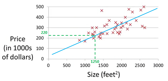
sizes that were sold for a range of different prices. Let's say that given this data set, you have a friend that's trying to sell a house and let's see if friend's house is size of 1250 square feet and you want to tell them how much they might be able to sell
the house for.
This is an example of a supervised learning algorithm. And it's supervised learning because we're given the, quotes, "right answer".
This is an example of a regression problem where the term regression refers to the fact that we are predicting a real-valued output namely the price.
different housing prices and our job is to learn from this data how to predict prices of the houses.
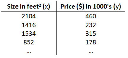
Training set of housing prices
Notation:
m= Number of training examples
x= “input” variable / features ( x here is a vector)
y= “output” variable / “target” variable (y here is a vector)
(x,y) - one training example
(x(i), y (i))-the ith training example,
x (1)=2014, x (3)=1534,y(1)=460,y(3)=315
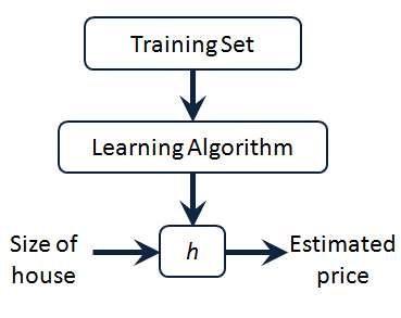
So here's how this supervised learning algorithm works. We saw that with the training set like our training set of housing prices and we feed that to our learning algorithm. Is the job of a learning algorithm to then output a
function which by convention is usually denoted lowercase h and h stands for hypothesis And what the job of the hypothesis is a function that takes as input the size of a house like maybe the size of the new house your friend's trying to sell so it takes in
the value of x and it tries to output the estimated value of y for the corresponding house. So h is a function that maps from x to y.
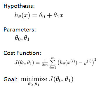
Our hypothesis function has the general form:
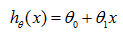
for shorthand sometimes hθ(x) is
denoted by h(x).
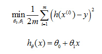
So then regression, what we're going to do is, I'm going to want to solve a minimization problem. So I'll write minimize overθ0, θ1. And I want this to be small. I want the difference between
h(x) and y to be small. And one thing I might do is try to minimize the square difference between the output of the hypothesis and the actual price of a house.
this is the prediction of my hypothesis when it is input to size of house number i. Minus the actual price that house number I was sold for, and I want to minimize the sum of my training set, sum from I equals one through M,
of the difference of this squared error, the square difference between the predicted price of a house, and the price that it was actually sold for. And just remind you of notation, m here was the size of my training set. So my m there is my number of training
examples. Right that hash sign is the abbreviation for number of training examples. And to make some of our, make the math a little bit easier, I'm going to actually look at we are 1 over m times that so let's try to minimize my average minimize one over 2m.
Putting the 2 at the constant one half in front, it may just sound the math probably easier so minimizing one-half of something, right, should give you the same values of the process, θ0, θ1, as minimizing that function.
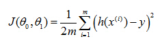
And just to rewrite this out a little bit more cleanly, what I'm going to do is, by convention we usually define acost function:
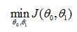
So the task is to minimize the cost function:
as a hypothesis with these parameters θ0, θ1, and with different choices of the parameters we end up with different straight line fits. So the data which are fit like so, and there's a cost function, and that was our
optimization objective.
value of cost function J(θ0,θ1) with different values ofθ0,
θ1
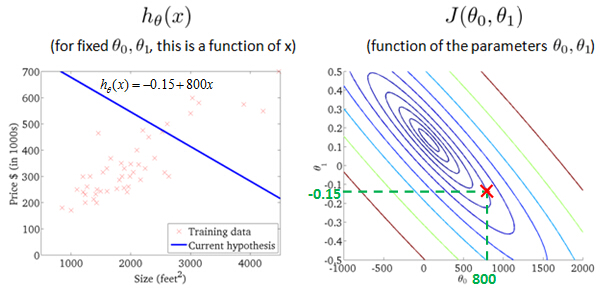
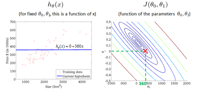
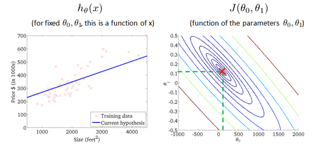
probably the best fits
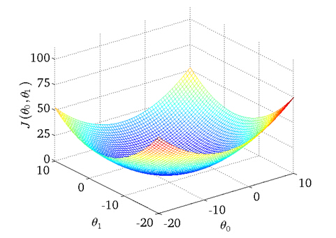
Imagine that we graph our hypothesis function based on its fields θ0 and θ1 (actually we are graphing the cost function for the combinations of parameters). This can be kind of confusing; we are moving up to a higher level of
abstraction. We are not graphing x and y itself, but the guesses of our hypothesis function.
We put θ0 on the x axis and θ1 on the z axis, with the cost function on the vertical y axis. The points on our graph will be the result of the cost function using our hypothesis with those specific theta parameters.
We will know that we have succeeded when our cost function is at the very bottom of the pits in our graph, i.e. when its value is the minimum.
The way we do this is by taking the derivative (the line tangent to a function) of our cost function. The slope of the tangent is the derivative at that point and it will give us a direction to move towards. We make steps down
that derivative by the parameter α, called the learning rate.
Start with some θ0 and θ1
Keep changing θ0 and θ1 to reduce J(θ0, θ1) until we hopefully end up at a minimum
The gradient descent equation is:
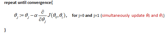
α is learning rate. Note that:
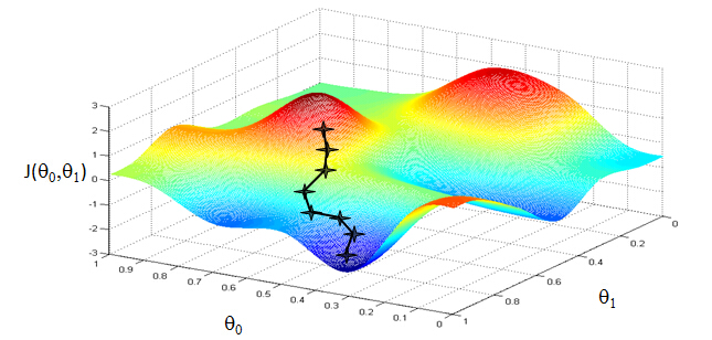
What does the Gradient Decent algorithm do is like the picture below:
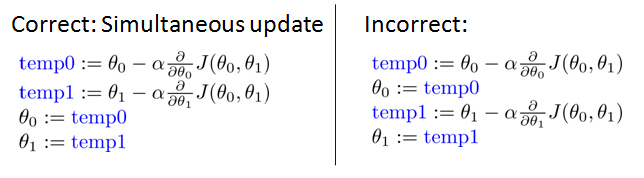
What we're going to do in gradient descent is we'll keep changingθ0 andθ1 a little bit to try to reduce
J(θ0, θ1), until hopefully, we wind at a minimum, or maybe at a local minimum. So let's see in pictures what gradient descent does.
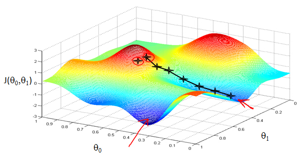
Gradient descent has an interesting property. This first time we ran gradient descent we were starting at this point over here. Started at that point over here. Now imagine we had initialized gradient descent just a couple steps
to the right. Imagine we'd initialized gradient descent with that point on the upper right. If you were to repeat this process, so start from that point, look all around, take a little step in the direction of steepest descent, you would do that. Then look
around, take another step, and so on. And if you started just a couple of steps to the right, gradient descent would've taken you to this second local optimum over on the right. So if you had started this first point, you would've wound up at this local optimum,
but if you started just at a slightly different location, you would've wound up at a very different local optimum. And this is a property of gradient descent.
derivation of the formulas are out of the scope of this course, but a really great one can be found here:
where m is the size of the training set, θ0 a constant that will be changing simultaneously with θ1 and x(i), y(i) are values of the given training set (data).
Note that we have separated out the two cases for θj and that for θ1 we are multiplying x(i) at the end due to the derivative.
The point of all this is that if we start with a guess for our hypothesis and then repeatedly
apply these gradient descent equations, our hypothesis will become more and more accurate.
function like gradient descent.
cost function and Gradient Descent algorithm to solve linear regression problem.
Linear Regression with One Variable
1. Model representation
Our first learning algorithm will be linear regression.Recall that in "regression problems", we are taking input variables and trying to map the output onto a "continuous" expected result function.
Linear regression with one variable is also known as "univariate linear regression."
Univariate linear regression is used when you want to predict a single output value from a single input value. We're doing supervised learning here, so that means we already have an idea what the input/output cause and effect
should be.
Example
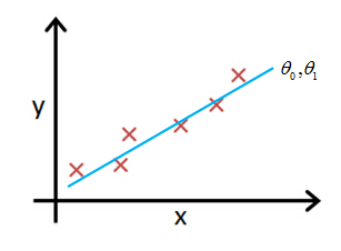
Let's use some motivating example of predicting housing prices. We're going to use a data set of housing prices from the city of Portland, Oregon. And here I'm going to plot my data set of a number of houses that were differentsizes that were sold for a range of different prices. Let's say that given this data set, you have a friend that's trying to sell a house and let's see if friend's house is size of 1250 square feet and you want to tell them how much they might be able to sell
the house for.
This is an example of a supervised learning algorithm. And it's supervised learning because we're given the, quotes, "right answer".
This is an example of a regression problem where the term regression refers to the fact that we are predicting a real-valued output namely the price.
Training set
More formally, in supervised learning, we have a data set and this data set is called a training set. So for housing prices example, we have a training set ofdifferent housing prices and our job is to learn from this data how to predict prices of the houses.
Training set of housing prices
Notation:
m= Number of training examples
x= “input” variable / features ( x here is a vector)
y= “output” variable / “target” variable (y here is a vector)
(x,y) - one training example
(x(i), y (i))-the ith training example,
x (1)=2014, x (3)=1534,y(1)=460,y(3)=315
The Hypothesis Function
So here's how this supervised learning algorithm works. We saw that with the training set like our training set of housing prices and we feed that to our learning algorithm. Is the job of a learning algorithm to then output a
function which by convention is usually denoted lowercase h and h stands for hypothesis And what the job of the hypothesis is a function that takes as input the size of a house like maybe the size of the new house your friend's trying to sell so it takes in
the value of x and it tries to output the estimated value of y for the corresponding house. So h is a function that maps from x to y.
Our hypothesis function has the general form:
for shorthand sometimes hθ(x) is
denoted by h(x).
2. Cost function
Idea: Choose θ0, θ1 so that hθ(x) is close to (x,y) for our training examples.So then regression, what we're going to do is, I'm going to want to solve a minimization problem. So I'll write minimize overθ0, θ1. And I want this to be small. I want the difference between
h(x) and y to be small. And one thing I might do is try to minimize the square difference between the output of the hypothesis and the actual price of a house.
this is the prediction of my hypothesis when it is input to size of house number i. Minus the actual price that house number I was sold for, and I want to minimize the sum of my training set, sum from I equals one through M,
of the difference of this squared error, the square difference between the predicted price of a house, and the price that it was actually sold for. And just remind you of notation, m here was the size of my training set. So my m there is my number of training
examples. Right that hash sign is the abbreviation for number of training examples. And to make some of our, make the math a little bit easier, I'm going to actually look at we are 1 over m times that so let's try to minimize my average minimize one over 2m.
Putting the 2 at the constant one half in front, it may just sound the math probably easier so minimizing one-half of something, right, should give you the same values of the process, θ0, θ1, as minimizing that function.
And just to rewrite this out a little bit more cleanly, what I'm going to do is, by convention we usually define acost function:
So the task is to minimize the cost function:
3. Cost function intuition
Let's look at some examples, to get back to intuition about what the cost function is doing, and why we want to use it. To recap, here's what we had last time. We want to fit a straight line to our data, so we had this formedas a hypothesis with these parameters θ0, θ1, and with different choices of the parameters we end up with different straight line fits. So the data which are fit like so, and there's a cost function, and that was our
optimization objective.
value of cost function J(θ0,θ1) with different values ofθ0,
θ1
probably the best fits
4. Gradient descent
So we have our hypothesis function and we have a way of measuring how accurate it is. Now what we need is a way to automatically improve our hypothesis function. That's where gradient descent comes in.Imagine that we graph our hypothesis function based on its fields θ0 and θ1 (actually we are graphing the cost function for the combinations of parameters). This can be kind of confusing; we are moving up to a higher level of
abstraction. We are not graphing x and y itself, but the guesses of our hypothesis function.
We put θ0 on the x axis and θ1 on the z axis, with the cost function on the vertical y axis. The points on our graph will be the result of the cost function using our hypothesis with those specific theta parameters.
We will know that we have succeeded when our cost function is at the very bottom of the pits in our graph, i.e. when its value is the minimum.
The way we do this is by taking the derivative (the line tangent to a function) of our cost function. The slope of the tangent is the derivative at that point and it will give us a direction to move towards. We make steps down
that derivative by the parameter α, called the learning rate.
Gradient descent algorithm
Outline:Start with some θ0 and θ1
Keep changing θ0 and θ1 to reduce J(θ0, θ1) until we hopefully end up at a minimum
The gradient descent equation is:
α is learning rate. Note that:
What does the Gradient Decent algorithm do is like the picture below:
What we're going to do in gradient descent is we'll keep changingθ0 andθ1 a little bit to try to reduce
J(θ0, θ1), until hopefully, we wind at a minimum, or maybe at a local minimum. So let's see in pictures what gradient descent does.
Gradient descent has an interesting property. This first time we ran gradient descent we were starting at this point over here. Started at that point over here. Now imagine we had initialized gradient descent just a couple steps
to the right. Imagine we'd initialized gradient descent with that point on the upper right. If you were to repeat this process, so start from that point, look all around, take a little step in the direction of steepest descent, you would do that. Then look
around, take another step, and so on. And if you started just a couple of steps to the right, gradient descent would've taken you to this second local optimum over on the right. So if you had started this first point, you would've wound up at this local optimum,
but if you started just at a slightly different location, you would've wound up at a very different local optimum. And this is a property of gradient descent.
Gradient Descent for Linear Regression
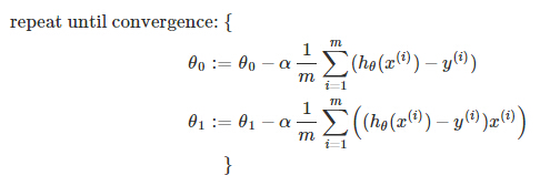
When specifically applied to the case of linear regression, a new form of the gradient descent equation can be derived. We can substitute our actual cost function and our actual hypothesis function and modify the equation to (thederivation of the formulas are out of the scope of this course, but a really great one can be found here:
where m is the size of the training set, θ0 a constant that will be changing simultaneously with θ1 and x(i), y(i) are values of the given training set (data).
Note that we have separated out the two cases for θj and that for θ1 we are multiplying x(i) at the end due to the derivative.
The point of all this is that if we start with a guess for our hypothesis and then repeatedly
apply these gradient descent equations, our hypothesis will become more and more accurate.
What's Next
Instead of using linear regression on just one input variable, we'll generalize and expand our concepts so that we can predict data with multiple input variables. Also, we'll solve for θ0 and θ1 exactly without needing an iterativefunction like gradient descent.

相关文章推荐
- Javascript SHA-1:Secure Hash Algorithm
- [转]可视化的数据结构和算法
- 统计文件中不小于某一长度的单词的个数(泛型算法实现)
- 使用他人的MD5编码类,修改形成密码串
- Extracting Structured Data from Web Pages
- (译)Cocos2d_for_iPhone_1_Game_Development_Cookbook:1.13使用CCTexture2DMutable调换调色盘
- Java中3DES加密
- Refactoring Notes-Refactoring Methods(3)
- 图书馆管理程序~~不过貌似功能!!有空再修修
- trainging contest#2(2011成都现场赛)I BY Hyoga
- C/C++头文件包含内容概览
- 堆栈的应用(1) 平衡符号 C++实现
- 程序员编程艺术第一章、左旋转字符串
- 程序员编程艺术:第三章续、Top K算法问题的实现
- 程序员编程艺术:第四章、现场编写类似strstr/strcpy/strpbrk的函数
- 十四、第三章再续:快速选择SELECT算法的深入分析与实现
- 程序员编程艺术:第七章、求连续子数组的最大和
- 程序员编程艺术:第八章、从头至尾漫谈虚函数
- 程序员编程艺术:第九章、闲话链表追赶问题
- 程序员编程艺术:第十章、如何给10^7个数据量的磁盘文件排序