基于轮廓的匹配算法(强,可在重叠堆积物体中识别)
2012-08-14 11:02
537 查看
(转)
这是一篇印度软件工程师的无私奉献!
非常具备参考价值!
如果能完成旋转匹配更接近于实用性.
当然要完成全角度匹配的难度是要量级数的提升.
Download source - 140 KB
Download demo - 138 KB
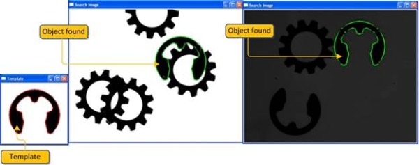
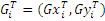
edge information for recognizing the object in the search image.
模块匹配:用一个模板图像在一幅未知位置的搜索图像中找到这个物体的位置。在本文中,我们实现了一个算法,用模板图像的边缘信息在搜索图像中搜索物体。
the algorithm should be computationally efficient. There are mainly two approaches to solve this problem, gray value based matching (or area based matching) and feature based matching (non area based).
由于模块匹配的速度和可靠性的原因,模块匹配实际是一个棘手的问题。当一个对象和其他对象混合时,此解决方案对于亮度变化匹配时健壮的,更重要的是,该算法应该是高效的。对于模块匹配问题,主要有基于灰度匹配(或地区建立匹配)和基于特征匹配(非面积为基础)。
Gray value based approach: In gray value based matching, the Normalized Cross Correlation (NCC) algorithm is known from old days. This is typically done
at every step by subtracting the mean and dividing by the standard deviation. The cross correlation of template t(x, y) with a sub image f(x, y) is:
基于灰度值的匹配:在基于灰度值的匹配中,规范化交叉相关(NCC)算法在过去已经给出,这个算法的特点就是在每一步中减去平均值并且通过标准差划分。模板图像t(x, y) 与子图像f(x, y)的互相关关系是:

Where n is the number of pixels in t(x, y) and f(x, y). [Wiki]
这里的n 是图像像素的个数。
Though this method is robust against linear illumination changes, the algorithm will fail when the object is partially visible or the object is mixed with other objects. Moreover, this algorithm is computationally expensive since
it needs to compute the correlation between all the pixels in the template image to the search image.
尽管这个算法对于线性照明的变化时健壮的,但是,当搜素图像部分与其他图像重叠时,这个算法将不能搜索到目标图像。同时,这个算法的计算量比较大,因为它需要计算搜索图像和目标图像所有像素点的互相关关系。
Feature based approach: Several methods of feature based template matching are being used in the image processing domain. Like edge based object recognition
where the object edges are features for matching, in Generalized Hough transform, an object’s geometric features will be used for matching.
特征点匹配:几种基于特征匹配的方法经常应用于图像的预处理。像基于边缘信息的匹配,在广义霍夫变换中,物体的几何特征也用于图像匹配。
In this article, we implement an algorithm that uses an object’s edge information for recognizing the object in a search image. This implementation uses the Open-Source Computer Vision library as a platform.
在本文中,我们实现一个算法,在搜索图像中,用一个物体的边缘信息识别这一物体。这个实现使用开源的计算机视觉库作为一个平台。
OpenCV can be downloaded free fromhere.OpenCV
(Open Source Computer Vision) is a library of programming functions for real time computer vision. Download OpenCV and install it in your system. Installation information can be read fromhere.
We need to configure our Visual Studio environment. This information can be read fromhere.
operation, computing an approximation of the gradient of the image intensity function.
在这里,首先介绍基于边缘信息的模块匹配技术。图像的亮度变化间断或急剧时,在一个数字图像中,边缘可以定义为一系列的点。从技术上讲,这是一个离散微分操作,计算一个梯度图像的近似的强度函数。
There are many methods for edge detection, but most of them can be grouped into two categories: search-based and zero-crossing based. The search-based methods detect edges by first computing a measure of edge strength, usually
a first-order derivative expression such as the gradient magnitude, and then searching for local directional maxima of the gradient magnitude using a computed estimate of the local orientation of the edge, usually the gradient direction. Here, we are using
such a method implemented by Sobel known as Sobel operator. The operator calculates thegradient of the image intensity at each point, giving the direction of the largest possible increase from light to dark and the rate of change in that direction.
有许多方法用于边缘检测,它们的绝大部分可以划分为两类:基于查找一类和基于零穿越的一类。(补:基于查找的方法通过寻找图像一阶导数中的最大和最小值来检测边界,通常是将边界定位在梯度最大的方向。基于零穿越的方法通过寻找图像二阶导数零穿越来寻找边界,通常是Laplacian过零点或者非线性差分表示的过零点。)基于搜索的边缘检测方法首先计算边缘强度, 通常用一阶导数表示, 例如梯度模,然后,用计算估计边缘的局部方向, 通常采用梯度的方向,并利用此方向找到局部梯度模的最大值。在这里,我们使用的是称为索贝尔算子。根据从亮到暗增长的最大可能性的方向和变化速率最快的方向,计算图像中每个点的梯度。
We are using these gradients or derivatives in X direction and Y direction for matching.
This algorithm involves two steps. First, we need to create an edge based model of the template image, and then we use this model to search in the search image.
我们在这里用梯度或者x方向和y方向的衍生来匹配。
这个算法包括两个步骤。首先,我们需要创建一个基于模板图像模型的边缘。然后,我们用这个边缘在搜索图像中寻找目标图像。
我们首先要从模板图像中创建数据集或者模板模型。
Here we are using a variation of Canny’s edge detection method to find the edges. You can read more on Canny’s edge detectionhere.
For edge extraction, Canny uses the following steps:
在这里,我们用一个变化中的Canny’s边缘检测方法来寻找边缘。对于边缘提取,Canny方法可以用以下步骤:


We are using an OpenCV function to find these values.
Once the edge direction is found, the next step is to relate the edge direction that can be traced in the image. There are four possible directions describing the surrounding pixels: 0 degrees, 45 degrees, 90 degrees, and 135
degrees. We assign all the directions to any of these angles.
一旦找到边缘的方向,下一步就是将边缘方向与图像中的被追踪的方向联系起来。这里有四种可能的方向来描述周围的像素点:0,45,90,135.我们将赋予其中的一个方向。
left and right pixel magnitudes. This will result in a thin image.
找到边缘方向后,我们要用非最大抑制算法处理。非最大抑制算法跟踪在这个方向上的左右像素点,如果该像素点小于左右像素点的值,那么就抑制该像素点。这将产生一个薄图像。
other edges can be traced through the image. While tracing an edge, we apply the lower threshold, allowing us to trace faint sections of edges as long as we find a starting point.
使用滞后门限需要两个阀值:高门限和低门限。我们应用高门限来标记处我们已经非常确定的边缘。从这些点出发,利用已经求出的方向信息,其它边缘也能求出。当我们在寻找边缘的时,可以通过低门限,只要我们找到了起始点就可以找到模糊的边缘。
边缘提取后,我们保存模板模型,即挑选出的边缘在x和y方向上的坐标信息。这些坐标将被重新安排来反映起始坐标(即重心)
centerOfGravity.y = CSum/noOfCordinates ; // center of gravity
// change coordinates to reflect center of gravity
for(int m=0;m<noOfCordinates ;m++)
{
int temp;
temp=cordinates[m].x;
cordinates[m].x=temp-centerOfGravity.x;
temp=cordinates[m].y;
cordinates[m].y =temp-centerOfGravity.y;
}

,
and its gradients in X and Y direction
, wherei = 1…n, n is the number
of elements in the Template (T) data set.
算法的下一个任务就是去寻找目标图像。我们已经知道了模板图像的一系列的边缘点和其在两个方向上的梯度。
We can also find the gradients in the search image (S)
,
where u = 1...number of rows in the search image, v = 1… number of columns in the search image.
In the matching process, the template model should be compared to the search image at all locations using a similarity measure. The idea behind similarity measure is to take the sum of all normalized dot products of gradient
vectors of the template image and search the image over all points in the model data set. This results in a score at each point in the search image. This can be formulated as follows:

接下来的工作就是利用已经求出的模版模型来寻找目标图像在搜索图像中。可以看到,在我们创建的模版图像中含有一系列的点
,在它的x和y的方向梯度,其中i=1..n,是模版图像的一系列点。
同样的,我们可以求出搜索图像的梯度。
在匹配过程中,模板模型与搜索图像在所有的像素点用一个相似的方法作对比。这个方法是将模板图像中的梯度向量归一化,然后通过模板图像的所有数据点来搜索图像。这个结果是搜索图像中每个点的得分。公式如下:
In case there is a perfect match between the template model and the search image, this function will return a score 1. The score corresponds to the portion of the object visible in the search image. In case the object is not
present in the search image, the score will be 0.
如果模板图像和搜索图像很好的匹配,这个函数将返回1。若对象不在搜索图像中,则返回0..
In practical situations, we need to speed up the searching procedure. This can be achieved using various methods. The first method is using the property of averaging. When finding the similarity measure, we need notevaluate
for all points in the template model if we can set a minimum score (Smin) for the similarity measure. For checking the partial score Su,v at a particular pointJ, we have to find the partial sum Sm. Sm at point m can be defines as
follows:
在有些情况下,我们需要加快处理速度。这里有很多方法来加速,第一种方法是使用属性的平均值。当发现一个相似的区域,如果通过相似方法设定了一个极小值,就不需要计算每个点的得分。为了检测在特定点J处的得分,我们必须找到sum部分和,SUM见如下定义:

It is evident that the remaining terms of the sum are smaller or equal to 1. So we can stop the evaluation if
.
很明显的可以看出,当部分和小于或等于一时,我们就可以停止计算
Another criterion can be that the partial score at any point should be greater than the minimum score. I.e.,

.
When this condition is used, matching will be extremely fast. But the problem is, if the missing part of the object is checked first, the partial sum will be low.In that case, that instance of the object will not be considered as a match. We can modify
this with another criterion where we check the first part of the template model with a safe stopping criteria and the remaining with a hard criteria,

.
The user can specify a greediness parameter (g) where the fraction of the template model is examined with a hard criteria. So that if g=1, all points in the template model are checked with the hard criteria, and if g=0, all the points will be checked with
a safe criteria only. We can formulate this procedure as follows.
The evaluation of the partial score can be stopped at:

This similarity measure has several advantages: the similarity measure is invariant to non-linear illumination changes because all gradient vectors are normalized. Since there is no segmentation on edge filtering, it will show
the true invariance against arbitrary changes in illumination. More importantly, this similarity measure is robust when the object is partially visible or mixed with other objects.
to the top of the pyramid. If the search is successful at this stage, the search is continued at the next level of the pyramid, which represents a higher resolution image. In this manner, the search is continued, and consequently, the result is refined until
the original image size, i.e., the bottom of the pyramid is reached.
Another enhancement is possible by extending the algorithm for rotation and scaling. This can be done by creating template models for rotation and scaling and performing search using all these template models
有各种各样的增强可能对于这个算法。为了进一步加速搜索过程,一个金字塔方法也可以使用。在这种情况下,搜索是开始在低分辨率与一个小图像的大小。这对应于金字塔的顶端。在这个阶段如果搜索成功,继续下一个级别的金字塔搜索,这代表了更高分辨率的图像。在这种方式下,搜索是持续的,因此,结果是精制直到原始图像大小,即,金字塔的底部是达到了。 另一个增强可以通过扩展算法,旋转和缩放。这可以通过创建模板模型的旋转和缩放和执行搜索使用所有这些模板模型。
Digital Image Processing [Rafael C. Gonzalez, Richard Eugene Woods]
http://dasl.mem.drexel.edu/alumni/bGreen/www.pages.drexel.edu/_weg22/can_tut.html
这是一篇印度软件工程师的无私奉献!
非常具备参考价值!
如果能完成旋转匹配更接近于实用性.
当然要完成全角度匹配的难度是要量级数的提升.
Download source - 140 KB
Download demo - 138 KB
Introduction
Template matching is an image processing problem to find the location of an object using a template image in another search image when its pose (X, Y, θ) is unknown. In this article, we implement an algorithm that uses an object’sedge information for recognizing the object in the search image.
模块匹配:用一个模板图像在一幅未知位置的搜索图像中找到这个物体的位置。在本文中,我们实现了一个算法,用模板图像的边缘信息在搜索图像中搜索物体。
Background
Template matching is inherently a tough problem due to its speed and reliability issues. The solution should be robust against brightness changes when an object is partially visible or mixed with other objects, and most importantly,the algorithm should be computationally efficient. There are mainly two approaches to solve this problem, gray value based matching (or area based matching) and feature based matching (non area based).
由于模块匹配的速度和可靠性的原因,模块匹配实际是一个棘手的问题。当一个对象和其他对象混合时,此解决方案对于亮度变化匹配时健壮的,更重要的是,该算法应该是高效的。对于模块匹配问题,主要有基于灰度匹配(或地区建立匹配)和基于特征匹配(非面积为基础)。
Gray value based approach: In gray value based matching, the Normalized Cross Correlation (NCC) algorithm is known from old days. This is typically done
at every step by subtracting the mean and dividing by the standard deviation. The cross correlation of template t(x, y) with a sub image f(x, y) is:
基于灰度值的匹配:在基于灰度值的匹配中,规范化交叉相关(NCC)算法在过去已经给出,这个算法的特点就是在每一步中减去平均值并且通过标准差划分。模板图像t(x, y) 与子图像f(x, y)的互相关关系是:
Where n is the number of pixels in t(x, y) and f(x, y). [Wiki]
这里的n 是图像像素的个数。
Though this method is robust against linear illumination changes, the algorithm will fail when the object is partially visible or the object is mixed with other objects. Moreover, this algorithm is computationally expensive since
it needs to compute the correlation between all the pixels in the template image to the search image.
尽管这个算法对于线性照明的变化时健壮的,但是,当搜素图像部分与其他图像重叠时,这个算法将不能搜索到目标图像。同时,这个算法的计算量比较大,因为它需要计算搜索图像和目标图像所有像素点的互相关关系。
Feature based approach: Several methods of feature based template matching are being used in the image processing domain. Like edge based object recognition
where the object edges are features for matching, in Generalized Hough transform, an object’s geometric features will be used for matching.
特征点匹配:几种基于特征匹配的方法经常应用于图像的预处理。像基于边缘信息的匹配,在广义霍夫变换中,物体的几何特征也用于图像匹配。
In this article, we implement an algorithm that uses an object’s edge information for recognizing the object in a search image. This implementation uses the Open-Source Computer Vision library as a platform.
在本文中,我们实现一个算法,在搜索图像中,用一个物体的边缘信息识别这一物体。这个实现使用开源的计算机视觉库作为一个平台。
Compiling the example code
We are using OpenCV 2.0 and Visual studio 2008 to develop this code. To compile the example code, we need to install OpenCV.OpenCV can be downloaded free fromhere.OpenCV
(Open Source Computer Vision) is a library of programming functions for real time computer vision. Download OpenCV and install it in your system. Installation information can be read fromhere.
We need to configure our Visual Studio environment. This information can be read fromhere.
The algorithm
Here, we are explaining an edge based template matching technique. An edge can be defined as points in a digital image at which the image brightness changes sharply or has discontinuities. Technically, it is a discrete differentiationoperation, computing an approximation of the gradient of the image intensity function.
在这里,首先介绍基于边缘信息的模块匹配技术。图像的亮度变化间断或急剧时,在一个数字图像中,边缘可以定义为一系列的点。从技术上讲,这是一个离散微分操作,计算一个梯度图像的近似的强度函数。
There are many methods for edge detection, but most of them can be grouped into two categories: search-based and zero-crossing based. The search-based methods detect edges by first computing a measure of edge strength, usually
a first-order derivative expression such as the gradient magnitude, and then searching for local directional maxima of the gradient magnitude using a computed estimate of the local orientation of the edge, usually the gradient direction. Here, we are using
such a method implemented by Sobel known as Sobel operator. The operator calculates thegradient of the image intensity at each point, giving the direction of the largest possible increase from light to dark and the rate of change in that direction.
有许多方法用于边缘检测,它们的绝大部分可以划分为两类:基于查找一类和基于零穿越的一类。(补:基于查找的方法通过寻找图像一阶导数中的最大和最小值来检测边界,通常是将边界定位在梯度最大的方向。基于零穿越的方法通过寻找图像二阶导数零穿越来寻找边界,通常是Laplacian过零点或者非线性差分表示的过零点。)基于搜索的边缘检测方法首先计算边缘强度, 通常用一阶导数表示, 例如梯度模,然后,用计算估计边缘的局部方向, 通常采用梯度的方向,并利用此方向找到局部梯度模的最大值。在这里,我们使用的是称为索贝尔算子。根据从亮到暗增长的最大可能性的方向和变化速率最快的方向,计算图像中每个点的梯度。
We are using these gradients or derivatives in X direction and Y direction for matching.
This algorithm involves two steps. First, we need to create an edge based model of the template image, and then we use this model to search in the search image.
我们在这里用梯度或者x方向和y方向的衍生来匹配。
这个算法包括两个步骤。首先,我们需要创建一个基于模板图像模型的边缘。然后,我们用这个边缘在搜索图像中寻找目标图像。
Creating an edge based template model
We first create a data set or template model from the edges of the template image that will be used for finding the pose of that object in the search image.我们首先要从模板图像中创建数据集或者模板模型。
Here we are using a variation of Canny’s edge detection method to find the edges. You can read more on Canny’s edge detectionhere.
For edge extraction, Canny uses the following steps:
在这里,我们用一个变化中的Canny’s边缘检测方法来寻找边缘。对于边缘提取,Canny方法可以用以下步骤:
Step 1: Find the intensity gradient of the image
Use the Sobel filter on the template image which returns the gradients in the X (Gx) and Y (Gy) direction. From this gradient, we will compute the edge magnitude and direction using the following formula:We are using an OpenCV function to find these values.
//第一步
cvSobel( src, gx, 1,0, 3 ); //gradient in X direction
cvSobel( src, gy, 0, 1, 3 ); //gradient in Y direction
for( i = 1; i < Ssize.height-1; i++ )
{
for( j = 1; j < Ssize.width-1; j++ )
{
_sdx = (short*)(gx->data.ptr + gx->step*i);
_sdy = (short*)(gy->data.ptr + gy->step*i);
fdx = _sdx[j]; fdy = _sdy[j]; // read x, y derivatives
//Magnitude = Sqrt(gx^2 +gy^2)
MagG = sqrt((float)(fdx*fdx) + (float)(fdy*fdy));
//Direction = invtan (Gy / Gx)
direction =cvFastArctan((float)fdy,(float)fdx);
magMat[i][j] = MagG;
if(MagG>MaxGradient)
MaxGradient=MagG; // get maximum gradient value for normalizing.
// get closest angle from 0, 45, 90, 135 set
if ( (direction>0 && direction < 22.5) || (direction >157.5 && direction < 202.5) || (direction>337.5 && direction<360) )
direction = 0;
else if ( (direction>22.5 && direction < 67.5) || (direction >202.5 && direction <247.5) )
direction = 45;
else if ( (direction >67.5 && direction < 112.5)|| (direction>247.5 && direction<292.5) )
direction = 90;
else if ( (direction >112.5 && direction < 157.5)|| (direction>292.5 && direction<337.5) )
direction = 135;
else
direction = 0;
orients[count] = (int)direction;
count++;
}
}
Once the edge direction is found, the next step is to relate the edge direction that can be traced in the image. There are four possible directions describing the surrounding pixels: 0 degrees, 45 degrees, 90 degrees, and 135
degrees. We assign all the directions to any of these angles.
一旦找到边缘的方向,下一步就是将边缘方向与图像中的被追踪的方向联系起来。这里有四种可能的方向来描述周围的像素点:0,45,90,135.我们将赋予其中的一个方向。
Step 2: Apply non-maximum suppression
After finding the edge direction, we will do a non-maximum suppression algorithm. Non-maximum suppression traces the left and right pixel in the edge direction and suppresses the current pixel magnitude if it is less than theleft and right pixel magnitudes. This will result in a thin image.
找到边缘方向后,我们要用非最大抑制算法处理。非最大抑制算法跟踪在这个方向上的左右像素点,如果该像素点小于左右像素点的值,那么就抑制该像素点。这将产生一个薄图像。
//第二步
for( i = 1; i < Ssize.height-1; i++ )
{
for( j = 1; j < Ssize.width-1; j++ )
{
switch ( orients[count] )
{
case 0:
leftPixel = magMat[i][j-1];
rightPixel = magMat[i][j+1];
break;
case 45:
leftPixel = magMat[i-1][j+1];
rightPixel = magMat[i+1][j-1];
break;
case 90:
leftPixel = magMat[i-1][j];
rightPixel = magMat[i+1][j];
break;
case 135:
leftPixel = magMat[i-1][j-1];
rightPixel = magMat[i+1][j+1];
break;
}
// compare current pixels value with adjacent pixels
if (( magMat[i][j] < leftPixel ) || (magMat[i][j] < rightPixel ) )
(nmsEdges->data.ptr + nmsEdges->step*i)[j]=0;
else
(nmsEdges->data.ptr + nmsEdges->step*i)[j]= (uchar)(magMat[i][j]/MaxGradient*255);
count++;
}
}
Step 3: Do hysteresis threshold
Doing the threshold with hysteresis requires two thresholds: high and low. We apply a high threshold to mark out thosee edges we can be fairly sure are genuine. Starting from these, using the directional information derived earlier,other edges can be traced through the image. While tracing an edge, we apply the lower threshold, allowing us to trace faint sections of edges as long as we find a starting point.
使用滞后门限需要两个阀值:高门限和低门限。我们应用高门限来标记处我们已经非常确定的边缘。从这些点出发,利用已经求出的方向信息,其它边缘也能求出。当我们在寻找边缘的时,可以通过低门限,只要我们找到了起始点就可以找到模糊的边缘。
int RSum=0,CSum=0;
int curX,curY;
int flag=1;

//Hysterisis threshold
for( i = 1; i < Ssize.height-1; i++ )
{
for( j = 1; j < Ssize.width; j++ )
{
_sdx = (short*)(gx->data.ptr + gx->step*i);
_sdy = (short*)(gy->data.ptr + gy->step*i);
fdx = _sdx[j]; fdy = _sdy[j];

MagG = sqrt(fdx*fdx + fdy*fdy); //Magnitude = Sqrt(gx^2 +gy^2)
DirG =cvFastArctan((float)fdy,(float)fdx);	 //Direction = tan(y/x)

////((uchar*)(imgGDir->imageData + imgGDir->widthStep*i))[j]= MagG;
flag=1;
if(((double)((nmsEdges->data.ptr + nmsEdges->step*i))[j]) < maxContrast)
{
if(((double)((nmsEdges->data.ptr + nmsEdges->step*i))[j])< minContrast)
{

(nmsEdges->data.ptr + nmsEdges->step*i)[j]=0;
flag=0; // remove from edge
////((uchar*)(imgGDir->imageData + imgGDir->widthStep*i))[j]=0;
}
else
{   // if any of 8 neighboring pixel is not greater than max contraxt remove from edge
if( (((double)((nmsEdges->data.ptr + nmsEdges->step*(i-1)))[j-1]) < maxContrast)	&&
(((double)((nmsEdges->data.ptr + nmsEdges->step*(i-1)))[j]) < maxContrast)		&&
(((double)((nmsEdges->data.ptr + nmsEdges->step*(i-1)))[j+1]) < maxContrast)	&&
(((double)((nmsEdges->data.ptr + nmsEdges->step*i))[j-1]) < maxContrast)		&&
(((double)((nmsEdges->data.ptr + nmsEdges->step*i))[j+1]) < maxContrast)		&&
(((double)((nmsEdges->data.ptr + nmsEdges->step*(i+1)))[j-1]) < maxContrast)	&&
(((double)((nmsEdges->data.ptr + nmsEdges->step*(i+1)))[j]) < maxContrast)		&&
(((double)((nmsEdges->data.ptr + nmsEdges->step*(i+1)))[j+1]) < maxContrast)	)
{
(nmsEdges->data.ptr + nmsEdges->step*i)[j]=0;
flag=0;
////((uchar*)(imgGDir->imageData + imgGDir->widthStep*i))[j]=0;
}
}

}
}
}
Step 4: Save the data set
After extracting the edges, we save the X and Y derivatives of the selected edges along with the coordinate information as the template model. These coordinates will be rearranged to reflect the start point as the center of gravity.边缘提取后,我们保存模板模型,即挑选出的边缘在x和y方向上的坐标信息。这些坐标将被重新安排来反映起始坐标(即重心)
// save selected edge information
curX=i;	curY=j;
if(flag!=0)
{
if(fdx!=0 || fdy!=0)
{
RSum=RSum+curX;	CSum=CSum+curY; // Row sum and column sum for center of gravity

cordinates[noOfCordinates].x = curX;
cordinates[noOfCordinates].y = curY;
edgeDerivativeX[noOfCordinates] = fdx;
edgeDerivativeY[noOfCordinates] = fdy;

//handle divide by zero
if(MagG!=0)
edgeMagnitude[noOfCordinates] = 1/MagG;  // gradient magnitude
else
edgeMagnitude[noOfCordinates] = 0;

noOfCordinates++;
}
}
centerOfGravity.x = RSum /noOfCordinates; // center of gravitycenterOfGravity.y = CSum/noOfCordinates ; // center of gravity
// change coordinates to reflect center of gravity
for(int m=0;m<noOfCordinates ;m++)
{
int temp;
temp=cordinates[m].x;
cordinates[m].x=temp-centerOfGravity.x;
temp=cordinates[m].y;
cordinates[m].y =temp-centerOfGravity.y;
}
Find the edge based template model
The next task in the algorithm is to find the object in the search image using the template model. We can see the model we created from the template image which contains a set of points:,
and its gradients in X and Y direction
, wherei = 1…n, n is the number
of elements in the Template (T) data set.
算法的下一个任务就是去寻找目标图像。我们已经知道了模板图像的一系列的边缘点和其在两个方向上的梯度。
We can also find the gradients in the search image (S)
,
where u = 1...number of rows in the search image, v = 1… number of columns in the search image.
In the matching process, the template model should be compared to the search image at all locations using a similarity measure. The idea behind similarity measure is to take the sum of all normalized dot products of gradient
vectors of the template image and search the image over all points in the model data set. This results in a score at each point in the search image. This can be formulated as follows:
接下来的工作就是利用已经求出的模版模型来寻找目标图像在搜索图像中。可以看到,在我们创建的模版图像中含有一系列的点
,在它的x和y的方向梯度,其中i=1..n,是模版图像的一系列点。
同样的,我们可以求出搜索图像的梯度。
在匹配过程中,模板模型与搜索图像在所有的像素点用一个相似的方法作对比。这个方法是将模板图像中的梯度向量归一化,然后通过模板图像的所有数据点来搜索图像。这个结果是搜索图像中每个点的得分。公式如下:
In case there is a perfect match between the template model and the search image, this function will return a score 1. The score corresponds to the portion of the object visible in the search image. In case the object is not
present in the search image, the score will be 0.
如果模板图像和搜索图像很好的匹配,这个函数将返回1。若对象不在搜索图像中,则返回0..
cvSobel( src, Sdx, 1, 0, 3 );  // find X derivatives
cvSobel( src, Sdy, 0, 1, 3 ); // find Y derivatives

// stoping criterias to search for model
double normMinScore = minScore /noOfCordinates; // precompute minumum score
double normGreediness = ((1- greediness * minScore)/(1-greediness)) /noOfCordinates; // precompute greedniness

for( i = 0; i < Ssize.height; i++ )
{
_Sdx = (short*)(Sdx->data.ptr + Sdx->step*(i));
_Sdy = (short*)(Sdy->data.ptr + Sdy->step*(i));

for( j = 0; j < Ssize.width; j++ )
{
iSx=_Sdx[j];  // X derivative of Source image
iSy=_Sdy[j];  // Y derivative of Source image

gradMag=sqrt((iSx*iSx)+(iSy*iSy)); //Magnitude = Sqrt(dx^2 +dy^2)

if(gradMag!=0) // hande divide by zero
matGradMag[i][j]=1/gradMag;   // 1/Sqrt(dx^2 +dy^2)
else
matGradMag[i][j]=0;

}
}
for( i = 0; i < Ssize.height; i++ )
{
for( j = 0; j < Ssize.width; j++ )
{
partialSum = 0; // initilize partialSum measure
for(m=0;m<noOfCordinates;m++)
{
curX	= i + cordinates[m].x ;	// template X coordinate
curY	= j + cordinates[m].y ; // template Y coordinate
iTx	= edgeDerivativeX[m];	// template X derivative
iTy	= edgeDerivativeY[m];    // template Y derivative

if(curX<0 ||curY<0||curX>Ssize.height-1 ||curY>Ssize.width-1)
continue;

_Sdx = (short*)(Sdx->data.ptr + Sdx->step*(curX));
_Sdy = (short*)(Sdy->data.ptr + Sdy->step*(curX));

iSx=_Sdx[curY]; // get curresponding  X derivative from source image
iSy=_Sdy[curY];// get curresponding  Y derivative from source image

if((iSx!=0 || iSy!=0) && (iTx!=0 || iTy!=0))
{
//partial Sum  = Sum of(((Source X derivative* Template X drivative) + Source Y derivative * Template Y derivative)) / Edge magnitude of(Template)* edge magnitude of(Source))
partialSum = partialSum + ((iSx*iTx)+(iSy*iTy))*(edgeMagnitude[m] * matGradMag[curX][curY]);

}

sumOfCoords = m + 1;
partialScore = partialSum /sumOfCoords ;
// check termination criteria
// if partial score score is less than the score than needed to make the required score at that position
// break serching at that coordinate.
if( partialScore < (MIN((minScore -1) + normGreediness*sumOfCoords,normMinScore*  sumOfCoords)))
break;

}
if(partialScore > resultScore)
{
resultScore = partialScore; //  Match score
resultPoint->x = i;			// result coordinate X
resultPoint->y = j;			// result coordinate Y
}
}
}
In practical situations, we need to speed up the searching procedure. This can be achieved using various methods. The first method is using the property of averaging. When finding the similarity measure, we need notevaluate
for all points in the template model if we can set a minimum score (Smin) for the similarity measure. For checking the partial score Su,v at a particular pointJ, we have to find the partial sum Sm. Sm at point m can be defines as
follows:
在有些情况下,我们需要加快处理速度。这里有很多方法来加速,第一种方法是使用属性的平均值。当发现一个相似的区域,如果通过相似方法设定了一个极小值,就不需要计算每个点的得分。为了检测在特定点J处的得分,我们必须找到sum部分和,SUM见如下定义:
It is evident that the remaining terms of the sum are smaller or equal to 1. So we can stop the evaluation if
.
很明显的可以看出,当部分和小于或等于一时,我们就可以停止计算
Another criterion can be that the partial score at any point should be greater than the minimum score. I.e.,
.
When this condition is used, matching will be extremely fast. But the problem is, if the missing part of the object is checked first, the partial sum will be low.In that case, that instance of the object will not be considered as a match. We can modify
this with another criterion where we check the first part of the template model with a safe stopping criteria and the remaining with a hard criteria,
.
The user can specify a greediness parameter (g) where the fraction of the template model is examined with a hard criteria. So that if g=1, all points in the template model are checked with the hard criteria, and if g=0, all the points will be checked with
a safe criteria only. We can formulate this procedure as follows.
The evaluation of the partial score can be stopped at:
// stoping criterias to search for model double normMinScore = minScore /noOfCordinates; // precompute minumum score double normGreediness = ((1- greediness * minScore)/(1-greediness)) /noOfCordinates; // precompute greedniness sumOfCoords = m + 1; partialScore = partialSum /sumOfCoords ; // check termination criteria // if partial score score is less than the score than // needed to make the required score at that position // break serching at that coordinate. if( partialScore < (MIN((minScore -1) + normGreediness*sumOfCoords,normMinScore* sumOfCoords))) break;
This similarity measure has several advantages: the similarity measure is invariant to non-linear illumination changes because all gradient vectors are normalized. Since there is no segmentation on edge filtering, it will show
the true invariance against arbitrary changes in illumination. More importantly, this similarity measure is robust when the object is partially visible or mixed with other objects.
Enhancements
There are various enhancements possible for this algorithm. For speeding up the search process further, a pyramidal approach can be used. In this case, the search is started at low resolution with a small image size. This correspondsto the top of the pyramid. If the search is successful at this stage, the search is continued at the next level of the pyramid, which represents a higher resolution image. In this manner, the search is continued, and consequently, the result is refined until
the original image size, i.e., the bottom of the pyramid is reached.
Another enhancement is possible by extending the algorithm for rotation and scaling. This can be done by creating template models for rotation and scaling and performing search using all these template models
有各种各样的增强可能对于这个算法。为了进一步加速搜索过程,一个金字塔方法也可以使用。在这种情况下,搜索是开始在低分辨率与一个小图像的大小。这对应于金字塔的顶端。在这个阶段如果搜索成功,继续下一个级别的金字塔搜索,这代表了更高分辨率的图像。在这种方式下,搜索是持续的,因此,结果是精制直到原始图像大小,即,金字塔的底部是达到了。 另一个增强可以通过扩展算法,旋转和缩放。这可以通过创建模板模型的旋转和缩放和执行搜索使用所有这些模板模型。
References
Machine Vision Algorithms and Applications [Carsten Steger, Markus Ulrich, Christian Wiedemann]Digital Image Processing [Rafael C. Gonzalez, Richard Eugene Woods]
http://dasl.mem.drexel.edu/alumni/bGreen/www.pages.drexel.edu/_weg22/can_tut.html
License
This article, along with any associated source code and files, is licensed underThe Code Project Open License (CPOL)About the Author
| Shiju PK Software Developer (Senior)  India Member  Follow on Twitter | I am a software engineer from India. my interests include coding, studying algorithms, image processing etc. |

相关文章推荐
- 基于轮廓的匹配算法(强,可在重叠堆积物体中识别)
- 人类是如何识别物体的呢,和图像学中基于特征的算法有什么异同?
- 基于OpenCV的目标物体颜色及轮廓的识别方法
- 使用SIFT和RANSAC算法,完成特征点的正确匹配,并求出变换矩阵,通过变换矩阵计算出要识别物体的边界
- 人类是如何识别物体的呢,和图像学中基于特征的算法有什么异同?
- 基于K-近邻算法识别手写数字的实现
- 字符串匹配算法 之 基于DFA(确定性有限自动机)的字符串模式匹配算法
- 串的模式匹配(基于KMP的匹配算法)
- 快速字符串模糊匹配--基于Horspool的模糊匹配算法
- 基于最小生成树的实时立体匹配算法简介
- 基于Shape Context的字符识别算法介绍
- 基于PHP实现栈数据结构和括号匹配算法示例
- 基于灰度的模板匹配算法(二):局部灰度值编码
- 基于灰度的模板匹配算法(一):MAD、SAD、SSD、MSD、NCC、SSDA、SATD算法
- 基于NCC模板匹配识别
- 游戏 匹配算法 实现(基于ELO分数、等待时长)
- 基于模板匹配的车牌识别系统实例
- 基于机器学习人脸识别face recognition具体的算法和原理
- Matlab图像处理学习笔记(三):基于匹配的目标识别
- 基于双数组的AC匹配算法学习