二、基本算法之DFS、BFS和A*
2012-06-11 13:16
991 查看
图中节点的遍历和搜索是老生常谈的话题,这里借由python的networkx库,复习一下之前的BFS和DFS,并对A*做一些理解。
1.BFS 广度优先搜索
其基本思想是优先从当前节点的邻居节点开始搜索,如果搜索不到,再搜索邻居的邻居。其在算法设计的时候,主要考虑节点的标记和邻居的保存
利用全局变量time进行计时,在pre列表中保存每个节点的父节点。
整体流程如下:
(i)从G中任取一个节点i,检查是否访问过了(可以通过检查相应的pre元素是否为-1)
(ii)初始化:将节点i放入一个双端队列visit_list
(Ⅲ)检验队列是否为空,不为空,则从左边取一个节点,将其尚未访问的所有邻居放入双端队列中(从右端放入),并设置邻居节点的父节点(假设为j)即pre[j]=i;如果队列为空,则算法结束
2.DFS 宽度优先搜索
其基本思想是随机邻居节点访问,如果邻居节点都访问过了,则回溯到其父节点,直到图中所有节点都被访问过了。
在visit_time中保存了每个节点访问的时间(从1开始),为了检验在图中有多少个环存在,特地设置了全局变量cycle_number,当从当前节点j搜索其邻居节点r时,如果发现邻居节点r已经被访问过了则存在环(这里假设没有自环存在)
整体过程:
(i)从图中任取节点i,如果节点i没有被访问,则到ii,否则如果图中所有节点都被访问过了则退出
(ii)将i设为访问过节点,寻找i的直接邻居r,如果邻居j没有被访问过,则将j的父节点设为r,并且重复ii
来自1986年的一篇论文P. E. Hart, N. J. Nilsson, and B. Raphael. A formal basis for the heuristic determination of minimum cost paths in graphs. IEEE Trans. Syst. Sci. and Cybernetics,
SSC-4(2):100-107。
A*搜寻算法
A*搜寻算法,俗称A星算法,作为启发式搜索算法中的一种,这是一种在图形平面上,有多个节点的路径,求出最低通过成本的算法。常用于游戏中的NPC的移动计算,或线上游戏的BOT的移动计算上。该算法像Dijkstra算法一样,可以找到一条最短路径;也像BFS一样,进行启发式的搜索。
A*算法最为核心的部分,就在于它的一个估值函数的设计上:
f(n)=g(n)+h(n)
其中f(n)是每个可能试探点的估值,它有两部分组成:
一部分,为g(n),它表示从起始搜索点到当前点的代价(通常用某结点在搜索树中的深度来表示)。
另一部分,即h(n),它表示启发式搜索中最为重要的一部分,即当前结点到目标结点的估值,
h(n)设计的好坏,直接影响着具有此种启发式函数的启发式算法的是否能称为A*算法。
一种具有f(n)=g(n)+h(n)策略的启发式算法能成为A*算法的充分条件是:
1、搜索树上存在着从起始点到终了点的最优路径。
2、问题域是有限的。
3、所有结点的子结点的搜索代价值>0。
4、h(n)=<h*(n) (h*(n)为实际问题的代价值)。
当此四个条件都满足时,一个具有f(n)=g(n)+h(n)策略的启发式算法能成为A*算法,并一定能找到最优解。
对于一个搜索问题,显然,条件1,2,3都是很容易满足的,而条件4: h(n)<=h*(n)是需要精心设计的,由于h*(n)显然是无法知道的,所以,一个满足条件4的启发策略h(n)就来的难能可贵了。
不过,对于图的最优路径搜索和八数码问题,有些相关策略h(n)不仅很好理解,而且已经在理论上证明是满足条件4的,从而为这个算法的推广起到了决定性的作用。且h(n)距离h*(n)的呈度不能过大,否则h(n)就没有过强的区分能力,算法效率并不会很高。对一个好的h(n)的评价是:h(n)在h*(n)的下界之下,并且尽量接近h*(n)。
A*算法和DFS、BFS有着较深关系,其中的g(n)和h(n)作为两个不同的代价,在DFS的搜索中,其关注的主要是邻居节点与当前节点的距离开销,此时可将g(n)认为是0;而在BFS中进行分层搜索时,以层次距离为主,此时可将h(n)认为是0。而且,当h(n)认为是0,则转换为单点源距离计算。
此外,对于f(n)的计算还有一些变种,例如f(n)=w*g(n)+(1-w)*h(n)、f(n)=g(n)+h(n)+h(n-1)等。(可以看到变种一个是增加维度,一个是修改计算比例)。
这里,对一个实例进行说明和实现:
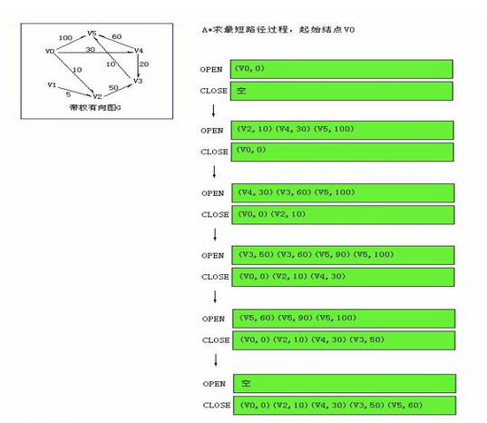
为了便于看到路径的形成,这里在python中用了两个列表,其中不仅保存了当前节点编号和权重,还保存了其前驱节点,这样也方便最后输出路径。
过程:
1.初始化列表open和close,将起点元素存入open中,其中open用来保存探索列表而close则保存访问列表
2.如果open不为空,则取出open的第一个元素,并转到2;如果open为空,则结束
3.取出第一个元素后,删除open中和第一个元素有相同目的节点的元素,并且对其邻居进行遍历,如果该邻居不在close中,则存入open中
4.对open中的节点按照f(n)大小进行升序排序,并转到2
可以清楚的看到5<-3<-4<-0,总计开销为60
相关参考和推荐:
http://blog.csdn.net/v_JULY_v/article/details/6111353
/article/5181102.html
http://as3.iteye.com/blog/841449
/article/10100693.html
1.BFS 广度优先搜索
其基本思想是优先从当前节点的邻居节点开始搜索,如果搜索不到,再搜索邻居的邻居。其在算法设计的时候,主要考虑节点的标记和邻居的保存
利用全局变量time进行计时,在pre列表中保存每个节点的父节点。
整体流程如下:
(i)从G中任取一个节点i,检查是否访问过了(可以通过检查相应的pre元素是否为-1)
(ii)初始化:将节点i放入一个双端队列visit_list
(Ⅲ)检验队列是否为空,不为空,则从左边取一个节点,将其尚未访问的所有邻居放入双端队列中(从右端放入),并设置邻居节点的父节点(假设为j)即pre[j]=i;如果队列为空,则算法结束
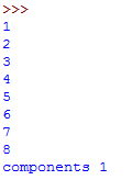
import networkx as nx
from collections import deque
def BFS_visit(i,G=nx.Graph(),visit_time=[],pre=[]):
global time
visit_list=deque()
visit_list.append(i)
while visit_list:
visit=visit_list.popleft()
print visit
time=time+1
visit_time[visit-1]=time
for node in G:
if G.has_edge(visit,node) and visit_time[node-1]==-1 and node not in visit_list:
visit_list.append(node)
pre[node-1]=visit

def BFS(G=nx.Graph()):
pre=[]
visit_time=[]
i=1
components=0
while i<=G.number_of_nodes():
pre.append(-1)
visit_time.append(-1)
i=i+1
for node in G.nodes():
if pre[node-1]==-1:
BFS_visit(node,G,visit_time,pre)
components=components+1
print 'components',components

time=0
G=nx.Graph()
G.add_edges_from([(1,2),(1,3),(2,4),(2,5),(3,6),(4,8),(5,8),(3,7)])
BFS(G)
运行的结果是
2.DFS 宽度优先搜索
其基本思想是随机邻居节点访问,如果邻居节点都访问过了,则回溯到其父节点,直到图中所有节点都被访问过了。
在visit_time中保存了每个节点访问的时间(从1开始),为了检验在图中有多少个环存在,特地设置了全局变量cycle_number,当从当前节点j搜索其邻居节点r时,如果发现邻居节点r已经被访问过了则存在环(这里假设没有自环存在)
整体过程:
(i)从图中任取节点i,如果节点i没有被访问,则到ii,否则如果图中所有节点都被访问过了则退出
(ii)将i设为访问过节点,寻找i的直接邻居r,如果邻居j没有被访问过,则将j的父节点设为r,并且重复ii
import networkx as nx
def DFS_visit(i,j,G=nx.Graph(),visit_time=[],pre=[]):
global time
global cycle_number
time=time+1
visit_time[j-1]=time
r=1
while r<=G.number_of_nodes():
if(G.has_edge(j,r) and visit_time[r-1]==-1):
pre[r-1]=j
DFS_visit(j,r,G,visit_time,pre)
elif(G.has_edge(j,r) and visit_time[r-1]!=-1 and visit_time[r-1]-1>visit_time[j-1]):
cycle_number=cycle_number+1
r=r+1
def DFS(G=nx.Graph()):
global cycle_number
visit_time=[]
pre=[]
i=1
while i<=G.number_of_nodes():
visit_time.append(-1)
pre.append(0)
i=i+1
print visit_time
i=1
components=0
while (i<=G.number_of_nodes() and visit_time[i-1]==-1):
DFS_visit(0,i,G,visit_time,pre)
components=components+1
i=i+1
visit_list=[]
i=1
while i<=G.number_of_nodes():
j=0
while j<G.number_of_nodes():
if visit_time[j]==i:
visit_list.append(j+1)
break
j=j+1
i=i+1
print 'visit order:',visit_time
print 'depth visit:',visit_list
print 'parent node:',pre
print 'components=',components
print 'cycle_number',cycle_number
cycle_number=0
time=0
G=nx.Graph()
G.add_edges_from([(1,2),(1,3),(2,4),(2,5),(3,6),(4,8),(5,8),(3,7)])
DFS(G)
3.A*算法
来自1986年的一篇论文P. E. Hart, N. J. Nilsson, and B. Raphael. A formal basis for the heuristic determination of minimum cost paths in graphs. IEEE Trans. Syst. Sci. and Cybernetics,
SSC-4(2):100-107。
A*搜寻算法
A*搜寻算法,俗称A星算法,作为启发式搜索算法中的一种,这是一种在图形平面上,有多个节点的路径,求出最低通过成本的算法。常用于游戏中的NPC的移动计算,或线上游戏的BOT的移动计算上。该算法像Dijkstra算法一样,可以找到一条最短路径;也像BFS一样,进行启发式的搜索。
A*算法最为核心的部分,就在于它的一个估值函数的设计上:
f(n)=g(n)+h(n)
其中f(n)是每个可能试探点的估值,它有两部分组成:
一部分,为g(n),它表示从起始搜索点到当前点的代价(通常用某结点在搜索树中的深度来表示)。
另一部分,即h(n),它表示启发式搜索中最为重要的一部分,即当前结点到目标结点的估值,
h(n)设计的好坏,直接影响着具有此种启发式函数的启发式算法的是否能称为A*算法。
一种具有f(n)=g(n)+h(n)策略的启发式算法能成为A*算法的充分条件是:
1、搜索树上存在着从起始点到终了点的最优路径。
2、问题域是有限的。
3、所有结点的子结点的搜索代价值>0。
4、h(n)=<h*(n) (h*(n)为实际问题的代价值)。
当此四个条件都满足时,一个具有f(n)=g(n)+h(n)策略的启发式算法能成为A*算法,并一定能找到最优解。
对于一个搜索问题,显然,条件1,2,3都是很容易满足的,而条件4: h(n)<=h*(n)是需要精心设计的,由于h*(n)显然是无法知道的,所以,一个满足条件4的启发策略h(n)就来的难能可贵了。
不过,对于图的最优路径搜索和八数码问题,有些相关策略h(n)不仅很好理解,而且已经在理论上证明是满足条件4的,从而为这个算法的推广起到了决定性的作用。且h(n)距离h*(n)的呈度不能过大,否则h(n)就没有过强的区分能力,算法效率并不会很高。对一个好的h(n)的评价是:h(n)在h*(n)的下界之下,并且尽量接近h*(n)。
A*算法和DFS、BFS有着较深关系,其中的g(n)和h(n)作为两个不同的代价,在DFS的搜索中,其关注的主要是邻居节点与当前节点的距离开销,此时可将g(n)认为是0;而在BFS中进行分层搜索时,以层次距离为主,此时可将h(n)认为是0。而且,当h(n)认为是0,则转换为单点源距离计算。
此外,对于f(n)的计算还有一些变种,例如f(n)=w*g(n)+(1-w)*h(n)、f(n)=g(n)+h(n)+h(n-1)等。(可以看到变种一个是增加维度,一个是修改计算比例)。
这里,对一个实例进行说明和实现:
为了便于看到路径的形成,这里在python中用了两个列表,其中不仅保存了当前节点编号和权重,还保存了其前驱节点,这样也方便最后输出路径。
过程:
1.初始化列表open和close,将起点元素存入open中,其中open用来保存探索列表而close则保存访问列表
2.如果open不为空,则取出open的第一个元素,并转到2;如果open为空,则结束
3.取出第一个元素后,删除open中和第一个元素有相同目的节点的元素,并且对其邻居进行遍历,如果该邻居不在close中,则存入open中
4.对open中的节点按照f(n)大小进行升序排序,并转到2
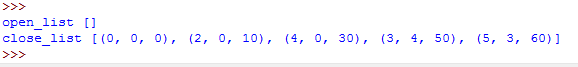
import networkx as nx
def Not_in(node, close_list=[]):
for item in close_list:
if item[0]==node:
return False
return True

def A_search(i,k,G=nx.DiGraph()):
open_list=[]
close_list=[]
open_list.append((i,0,0))
while open_list:
item=open_list[0]
del open_list[0]
boo=1
while(boo and open_list):
i=0
boo=0
while i<len(open_list):
if open_list[i][0]==item[0]:
del open_list[i]
boo=1
i=i+1
close_list.append(item)
if item[0]==k:
print 'open_list',open_list
print 'close_list',close_list
break
for node in G.nodes():
if G.has_edge(item[0],node) and Not_in(node,close_list):
weight=G.get_edge_data(item[0],node)['weight']+item[2]
open_list.append((node,item[0],weight))
open_number=len(open_list)
i=1
while i<=open_number:
j=0
while j<=open_number-i-1:
if open_list[j+1][2]<open_list[j][2]:
item=open_list[j]
open_list[j]=open_list[j+1]
open_list[j+1]=item
j=j+1
i=i+1

G=nx.DiGraph()
G.add_weighted_edges_from([(0,5,100),(0,2,10),(0,4,30),(1,2,5),(2,3,50),(3,5,10),(4,3,20),(4,5,60)])
A_search(0,5,G)
输出为:
可以清楚的看到5<-3<-4<-0,总计开销为60
相关参考和推荐:
http://blog.csdn.net/v_JULY_v/article/details/6111353
/article/5181102.html
http://as3.iteye.com/blog/841449
/article/10100693.html

相关文章推荐
- 图的基本算法(BFS和DFS)
- 图的基本算法(BFS和DFS)
- 基本图算法: BFS和DFS---shortest path和topological sort
- 基本算法DFS以及BFS
- 图的基本算法(BFS和DFS)
- 图算法(一)——基本图算法(BFS,DFS及其应用)(1)
- 图算法(一)——基本图算法(BFS,DFS及其应用)(2)
- 图的基本算法(BFS和DFS)
- 图的基本算法(BFS和DFS)
- 图的基本算法(BFS和DFS)转载自https://www.jianshu.com/p/70952b51f0c8
- 图的基本算法--深度优先搜索(dfs) 和 广度优先搜索(bfs)
- 图基本算法 拓扑排序(基于邻接表的dfs实现)
- 无向图的DFS和BFS算法实现
- 算法学习笔记 二叉树和图遍历—深搜 DFS 与广搜 BFS
- 图的DFS和BFS算法解析
- 算法总结(12)--dfs, bfs记忆化, 减少不必要的搜索
- BFS和DFS算法分析对比及优化
- BFS/DFS算法介绍与实现
- Stanford 算法入门 Week 4 Graph,BFS,DFS, partial_sort
- 算法--全排列、全子集、DFS\BFS问题